5 Data Exchanged with the Coupler

Each component model exchanges data with the coupler only. Component models have no direct connection with each other - all data is routed through the coupler. Most data is in the form of 2D fields. This data is accompanied by certain timing and control information (arrays of scalar real or integer values), such as the current simulation data and time.

5.1 Units Convention

All data exchanged conforms to this units convention:

Sign convention:
     positive value <=> downward flux

Unit convention:
     temperature   ~ Kelvin
     salt          ~ g/kg 
     velocity      ~ m/s
     pressure      ~ N/m^2 = Pa
     humidity      ~ kg/kg
     air density   ~ kg/m^3
     momentum flux ~ N/m^2
     heat flux     ~ W/m^2
     water flux    ~ (kg/s)/m^2
     salt flux     ~ (kg/s)/m^2
     coordinates   ~ degrees north or east
     area          ~ radians^2
     domain mask   ~ 0 <=> an inactive grid cell

5.2 Time Invariant Data

This section provides a list of the time invariant data exchanged between the coupler and each component model. Generally this data is the "domain" data: coordinate arrays, domain mask, cell areas, etc. It is assumed that the domain of all models is represented by a 2D array (although not necessarily a latitude/longitude grid).

5.2.1 Data Sent to Coupler

     domain data
   * grid cell's center coordinates, zonal      (degrees north)
   * grid cell's center coordinates, meridional (degrees east)
   * grid cell's four vertex coordinates, zonal      (degrees north)
   * grid cell's four vertex coordinates, meridional (degrees east)
   * grid cell area (radians squared)
   * grid cell domain mask ( 0 <=> not in active domain)
   * ni,nj: the dimensions of the underlying 2D array data structure

     time coordination data
   * ncpl: number of times per day the component will communicate (exchange 
     data) with the coupler.

     other information
   * IC flag: indicates whether the coupler should use model IC's contained
     on the coupler's restart file or IC's in the initial message sent from
     the component model.

5.2.2 Data Received from Coupler

     time coordination data
   * date, seconds: the exact time the coupler will start the simulation from.

5.3 Time Variant Data

This section provides a list of the time-evolving data sent exchanged between the coupler and the data model. Generally this is state, flux, and diagnostic quantities.

Each data model provides the coupler with a set of output fields. Output fields from a model include output states (which can be used by another component to compute fluxes) and output fluxes (fluxes that were computed within the model and which need to be exchanged with another component model).

The coupler provides each component model with input fields. Input fields sent to a model include input states (the state variables of other models, which are needed to do a flux calculation) and input fluxes (a forcing fields computed by some other component).

Flux fields sent to or from the coupler are understood to apply over the communication interval beginning when the data was received and ending when the next message is received. The data models must insure that fluxes sent to the coupler are appropriate in this context.

5.3.1 Data Sent to Coupler

     states
   * ice fraction
   * surface temperature (Kelvin)
   * albedo: visible      , direct  
   * albedo: near-infrared, direct  
   * albedo: visible      , diffuse 
   * albedo: near-infrared, diffuse 

     fluxes
   * atm/ice: zonal      surface stress (N/m^2)
   * atm/ice: meridional surface stress (N/m^2)
   * atm/ice: latent heat                (W/m^2)
   * atm/ice: sensible heat              (W/m^2)
   * atm/ice: longwave radiation, upward (W/m^2)
   * atm/ice: evaporation ((kg/s)/m^2)
   * ice/ocn: penetrating shortwave radiation (W/m^2)
   * ice/ocn: ocean heat used for melting (W/m^2)
   * ice/ocn: melt water ((kg/s)/m^2)
   * ice/ocn: salt flux  ((kg/s)/m^2)
   * ice/ocn: zonal      surface stress (N/m^2)
   * ice/ocn: meridional surface stress (N/m^2)

     diagnostic quantities
   * net shortwave radiation (W/m^2)
   * 2 meter reference air temperature (Kelvin)

5.3.2 Data Received from Coupler

     states
   * ocn: temperature (Kelvin)
   * ocn: salinity    (g/kg)
   * ocn: zonal      velocity (m/s)
   * ocn: meridional velocity (m/s)
   * atm: layer height (m)
   * atm: zonal      velocity (m/s)
   * atm: meridional velocity (m/s)
   * atm: potential temperature (Kelvin)
   * atm: temperature           (Kelvin)
   * atm: specific humidity (kg/kg)
   * atm: density (kg/m^3)

     fluxes
   * ocn: dh/dx: zonal      surface slope (m/m)
   * ocn: dh/dy: meridional surface slope (m/m)
   * ocn: Q>0: heat of fusion    (W/m^2), or
          Q<0: melting potential (W/m^2)
   * atm: shortwave radiation: downward, visible      , direct  (W/m^2)
   * atm: shortwave radiation: downward, near-infrared, direct  (W/m^2)
   * atm: shortwave radiation: downward, visible      , diffuse (W/m^2)
   * atm: shortwave radiation: downward, near-infrared, diffuse (W/m^2)
   * atm: longwave  radiation, downward (W/m^2)
   * atm: precipitation: liquid ((kg/s)/m^2)
   * atm: precipitation: frozen ((kg/s)/m^2)

5.3.3 How Output Data is Derived

Ice extent (fractional coverage at each grid cell) is obtained by reading in climatological monthly mean ice fraction data from an input data file and linear interpolation in time.

The ice surface temperature is computed according to a formula that roughly approximates the ice temperature found in standalone versions of CCM2 (an older version of the CCSM atmosphere component). The formula is (for the northern hemisphere):

$$T_{ice} = 260 + 10 cos(2 \pi (rmonth - 8)/12)$$

where rmonth = 0 corresponds to January 1st, and rmonth = 6 corresponds to July 1st.

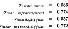
Surface albedos sent to the coupler are somewhat arbitrary but are based on reasonable values for snow and ice albedos combined with an assumption about the fraction of surface snow vs. ice. The albedo values are:

$$\begin{eqnarray*} \alpha_{visible, direct} &=& 0.586 \\ \alpha_{near-infrared, ... ...diffuse} &=& 0.557 \\ \alpha_{near-infrared, diffuse} &=& 0.772 \end{eqnarray*}$$

The atmosphere/ice sensible, latent, and upward-longwave heat fluxes, evaporation, surface stress, and 2-meter reference temperatures are calculated according to an involved formula that is documented in the CCSM2.0.1 Coupler (cpl5) document. See that document for details. The Coupler does a similar calculation for atmosphere/ocean fluxes.

The default value of penetrating short-wave radiation is zero. Optionally, by changing the namelist parameter flux_swpf ("short-wave penetrating factor"), will allow an arbitrary fraction of net solar absorbed to pass through the ice component and be absorbed into the ocean below.

Melt water is set to zero by default. Optionally, the flux_acc namelist parameter activates the dice5 model's ability to accumulate ice formed in the ocean component. This ice formed is flux field sent from the ocean to the ice. This accumulated ice can subsequently be melted back into the ocean component if and when there is sufficient melting potential. Melting potential is also a field sent from the ocean to the ice component.

Salt flux is alway set to zero.

The ice/ocean surface stress is set equal to the atmosphere/ice surface stress (see above).