Table of Contents
List of Figures
Table of Contents
This manual is intended for anyone who plans to get their hands dirty modifying CAM code. It is a work in progress! So despite our best intentions to provide exactly what you need to know in order to add your new science or diagnostic capability to CAM, undoubtedly we will fall short. If you don't find the information you need here, then please post to the CESM bulletin board using the CAM forum for MAKING CHANGES TO THE SOURCE CODE .
The following list contains the topics we hope to address... eventually.
CAM's high level architecture
interface design for the dynamics and physics packages
utilities for the dynamics and physics packages
driver layers
top level data structures for physics and dynamics
coupling between the physics and dynamics packages
infrastructure utilities (e.g., output and time management)
design of the configure and build-namelist utilities
CAM must produce high quality simulations for use in a wide variety of activities, for example:
as the atmosphere component of CESM it is used for studying climate change and climate variability, and to produce simulations for national and international assessment activities;
as the atmosphere component of data assimilation systems (e.g., DART) it must make accurate weather and constituent transport forecasts;
as a standalone model it is used for research in the development of new dynamical cores and parameterizations of subgrid-scale physics and chemistry.
The use of CAM in climate research and assessment activities, and for data assimilation requires high performance, which must be achievable on a wide variety of computer architectures.
The use of CAM in research and development environments requires that its design be modular to facilitate change, and the addition of new functionality.
One consequence of being a community effort is that CAM has a large and diverse group of developers. We also include code that was not written specifically for CAM. Hence the contributed CAM code base does not conform to any consistent standard, and the project has never had the resources to attempt to enforce a standard.
The purpose of coding conventions is to facilitate the production of readable, testable, and maintainable code. Taking into account the realities of how CAM's code has been developed, our approach to coding conventions is to allow considerable flexibility in matters of style, and to encourage best coding practices on matters of substance. Our current thoughts on this are maintained on this wiki page.
Table of Contents
At the highest level CAM is designed to be a component in an Earth system model. This architecture requires each component to provide initialize, run, and finalize methods, along with import and export state objects designed to allow communication with other other components mediated by a coupling component. The coupling component acts as the system driver and provides capabilities such as mapping between different component grids, merging from several source components to a destination component, computation of physical quantities such as fluxes which require input from multiple components, and the computation of diagnostics. The CESM uses the CPL7 coupling component which is documented here, and described in the paper Craig et al.[2012].
The CAM component employs a modular design to provide flexibility in incorporating new dynamical cores and parameterized physics packages. The design allows the dynamical core and the physics package to use different grids and/or different grid decompositions, and uses an internal dynamics-physics coupler which is independent of the high level coupler for the Earth system components. It contains a multi-level approach to the physics driver layers which facilitates supporting multiple physics packages, both new and old, from the same code base. And it provides physics infrastructure services that help coordinate the actions of the various physics packages.
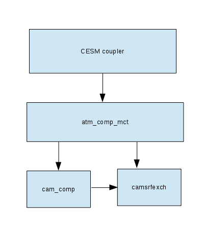
The CAM component interface is implemented in two layers. This architecture insulates the CAM specific data structures used by the import and export state objects from the data structures used by the coupling component. The modules that implement this design are outlined in Figure 3.1, “Component Interface Dependencies”.
Figure 3.1. Component Interface Dependencies
Modules at the tails of the arrows depend on the modules at the heads of
the arrows.
The CAM component interface is implemented in the following modules:
-
atm_comp_mct The
atm_comp_mctmodule is a translation layer which implements the generic atmosphere component interfaces required by CPL7 using the CAM component interfaces provided bycam_compand the CAM import and export state objects provided bycamsrfexch.atm_comp_mctdoes the translation between the MCT data structures used by the coupler and CAM's data structures.-
cam_comp The
cam_compmodule provides CAM's component interfaces, i.e., the initial, run, and final methods.-
camsrfexch The
camsrfexchmodule provides CAM's import and export state objects.
Table of Contents
The top level physics drivers are phys_run1 and phys_run2. These
subroutines call subordinate drivers which split the physics packages into
two groups. The first group managed by the driver tphysbc is called
before the coupling with surface processes, while the second group managed
by the driver tphysac is called after coupling.
The fundamental data structure used by the physics driver was designed for
performance on a wide range of computer architectures. It can be tuned for
vector or non-vector systems, to provide load balancing while minimizing
communication overhead, and to exploit the optimal mix of distributed
Message Passing Interface (MPI) processes and shared OpenMP threads
Worley et al. [2005]. The data structure contains an arbitrary
collection of vertical columns, and is referred to as a "chunk." There are
no assumptions about the horizonal locations of the columns, e.g., they are
not necessarily neighbors in the global grid. The chunks are defined in
the module phys_grid which provides query functions that return the
number of columns in each chunk and the latitude, longitude coordinates of
the individual columns in a chunk. The "physics grid" decomposition is a
collection of disjoint chunks, i.e., each column in the global grid is
contained in exactly one chunk.
SPMD parallelism is achieved by allocating a subset of the chunks that
comprise the physics grid to each MPI process. In each MPI process the
physics driver may optionally perform SMP parallelism by distributing the
calculations on these chunks among the available threads. The calls to
tphysbc and tphysac are inside threaded loops. A single call
to either tphysbc or tphysac passes only a single chunk of
the decomposed physics grid, and this data is then passed to the individual
physics packages.
The data on a chunk of the physics grid which is passed to a physics
package interface routine is actually a variable of a derived type that
contains multiple fields defined on a chunk. Several derived types are
defined in module physics_types. The type physics_state
contains fields that define the physics state. A variable of this type is
passed with intent in to the individual physics packages to enforce
the requirement that a physics package may not directly modifiy the model
state. The type physics_ptend contains fields that represent the
tendencies to state variables from an individual parameterization. A
variable of this type is passed with intent out from the individual
physics packages. The update of the physics state is done by the method
physics_update which is part of the physics_types module.
A call to physics_update is made after each call to a physics
package so that the state and/or the total physics tendency may be updated.
The derived type that contains the fields for the total physics tendency is
physics_tend.
Information not contained in the state structure may be communicated between parameterizations and across time steps using the physics buffer utility module. This module handles all issues of allocating space, cycling time levels, and reading and writing restart information for data in the buffer.
Array dimensions for chunks (pcols and pver) are from the module
ppgrid. The array dimension for advected constituents (pcnst) is from
the module constituents. Currently the parameters pcols, pver, and
pcnst are set by the cpp macros PCOLS, PLEV, and PCNST during the
build process.
integer, parameter ::&
   pcols = PCOLS, &! maximum number of columns in a chunk
   pver  = PLEV,  &! number of vertical levels
   pcnst = PCNST   ! number of advected constituents
Note that currently CAM uses the same number of vertical levels in both the dynamics and physics grid. But the data structures allow the flexibility to change this in the future.
The precision of real data passing through the interface is specified by
the kind parameter shr_kind_r8 in module shr_kind_mod. This
value is set to give 8-byte floating point representations. At the top of
most CAM modules will be the following code segment which provides the
shorthand notation, r8, as a convenience for shorter type
declaration statements.
use shr_kind_mod, only: r8 => shr_kind_r8
The argument lists of the public interface methods are insulated from changes in the specific fields that may need to be passed through them by encapsulating the fields in several derived data types. The components of these types use the chunk data structure.
The physics driver stores the physics state using the derived type,
physics_state which is defined in the physics_types module. The
physics_state type contains the state variables as well as variables
derived from the state that are passed between the physics and dynamics.
Memory for an array of physics state objects (each object stores a single
"chunk" of data) is allocated by the physics_type_alloc routine called
from phys_init. The state data from the dynamical core (stored in dycore
specific data structures) is rearranged to the physics data structure by
the d_p_coupling routine, and is passed as input to the top level physics
driver phys_run1 from where it is subsequently passed through the
interface subroutines of the individual packages. A package is not
allowed to change the values of these fields. A package which is designed
to directly change its input state must use a local copy of the appropriate
input fields.
The physics state derived type is defined as follows:
  type physics_state
     integer                                     :: &
          lchnk,                &! chunk index
          ngrdcol,              &! -- Grid        -- number of active columns (on the grid)
          nsubcol(pcols),       &! -- Sub-columns -- number of active sub-columns in each grid column
          psetcols=0,           &! --             -- max number of columns set - if subcols = pcols*psubcols, else = pcols
          ncol=0,               &! --             -- sum of nsubcol for all ngrdcols - number of active columns
          indcol(pcols*psubcols) ! --             -- indices for mapping from subcols to grid cols
     real(r8), dimension(:), allocatable         :: &
          lat,     &! latitude (radians)
          lon,     &! longitude (radians)
          ps,      &! surface pressure
          psdry,   &! dry surface pressure
          phis,    &! surface geopotential
          ulat,    &! unique latitudes  (radians)
          ulon      ! unique longitudes (radians)
     real(r8), dimension(:,:),allocatable        :: &
          t,       &! temperature (K)
          u,       &! zonal wind (m/s)
          v,       &! meridional wind (m/s)
          s,       &! dry static energy
          omega,   &! vertical pressure velocity (Pa/s)
          pmid,    &! midpoint pressure (Pa)
          pmiddry, &! midpoint pressure dry (Pa)
          pdel,    &! layer thickness (Pa)
          pdeldry, &! layer thickness dry (Pa)
          rpdel,   &! reciprocal of layer thickness (Pa)
          rpdeldry,&! recipricol layer thickness dry (Pa)
          lnpmid,  &! ln(pmid)
          lnpmiddry,&! log midpoint pressure dry (Pa)
          exner,   &! inverse exner function w.r.t. surface pressure (ps/p)^(R/cp)
          zm        ! geopotential height above surface at midpoints (m)

     real(r8), dimension(:,:,:),allocatable      :: &
          q         ! constituent mixing ratio (kg/kg moist or dry air depending on type)

     real(r8), dimension(:,:),allocatable        :: &
          pint,    &! interface pressure (Pa)
          pintdry, &! interface pressure dry (Pa)
          lnpint,  &! ln(pint)
          lnpintdry,&! log interface pressure dry (Pa)
          zi        ! geopotential height above surface at interfaces (m)

     real(r8), dimension(:),allocatable          :: &
          te_ini,  &! vertically integrated total (kinetic + static) energy of initial state
          te_cur,  &! vertically integrated total (kinetic + static) energy of current state
          tw_ini,  &! vertically integrated total water of initial state
          tw_cur    ! vertically integrated total water of new state
     integer :: count ! count of values with significant energy or water imbalances
     integer, dimension(:),allocatable           :: &
          latmapback, &! map from column to unique lat for that column
          lonmapback, &! map from column to unique lon for that column
          cid        ! unique column id
     integer :: ulatcnt, &! number of unique lats in chunk
                uloncnt   ! number of unique lons in chunk

     ! Whether allocation from dycore has happened.
     logical :: dycore_alloc = .false.

     ! WACCM variables set by dycore
     real(r8), dimension(:,:),allocatable        :: &
          uzm,     &  ! zonal wind for qbo (m/s)
          frontgf, &  ! frontogenesis function
          frontga     ! frontogenesis angle

  end type physics_state
The physics_ptend type stores tendencies and their associated
boundary fluxes for a single package. A variable of this type is an intent
out argument to the CAM interface for each package. In the
driver layer these objects are passed to the physics_update routine which
is called after each package and used to update state and
accumulated tendency objects.
The package tendency derived type is defined as follows:
  type physics_ptend

     integer   ::   psetcols=0 ! max number of columns set- if subcols = pcols*psubcols, else = pcols

     character*24 :: name    ! name of parameterization which produced tendencies.

     logical ::             &
          ls,               &! true if dsdt is returned
          lu,               &! true if dudt is returned
          lv                &! true if dvdt is returned

     logical,dimension(pcnst) ::  lq = .false.  ! true if dqdt() is returned

     integer ::             &
          top_level,        &! top level index for which nonzero tendencies have been set
          bot_level          ! bottom level index for which nonzero tendencies have been set

     real(r8), dimension(:,:),allocatable   :: &
          s,                &! heating rate (J/kg/s)
          u,                &! u momentum tendency (m/s/s)
          v                  ! v momentum tendency (m/s/s)
     real(r8), dimension(:,:,:),allocatable :: &
          q                  ! consituent tendencies (kg/kg/s)

     ! boundary fluxes
     real(r8), dimension(:),allocatable     ::&
          hflux_srf,     &! net heat flux at surface (W/m2)
          hflux_top,     &! net heat flux at top of model (W/m2)
          taux_srf,      &! net zonal stress at surface (Pa)
          taux_top,      &! net zonal stress at top of model (Pa)
          tauy_srf,      &! net meridional stress at surface (Pa)
          tauy_top        ! net meridional stress at top of model (Pa)
     real(r8), dimension(:,:),allocatable   ::&
          cflx_srf,      &! constituent flux at surface (kg/m2/s)
          cflx_top        ! constituent flux top of model (kg/m2/s)

  end type physics_ptend
The physics driver stores the accumulated tendencies from all of the
individual physics packages using the tendency structure physics_tend
which is defined in the physics_types module. The physics_tend type
stores the tendencies that are passed from the physics to the dynamics.
Memory for an array of physics tendency objects is allocated in the same
place as the memory for the state objects. The array is passed to the top
level physics drivers, however, unlike the state objects, the accumulated
tendency objects are not passed to individual physics packages. Instead it
is updated in the driver code by the physics_update routine after the
call to each of the physics packages returns its own tendencies.
The physics tendency derived type is defined as follows:
  type physics_tend

     integer   ::   psetcols=0 ! max number of columns set- if subcols = pcols*psubcols, else = pcols

     real(r8), dimension(:,:),allocatable        :: dtdt, dudt, dvdt
     real(r8), dimension(:),  allocatable        :: flx_net
     real(r8), dimension(:),  allocatable        :: &
          te_tnd,  &! cumulative boundary flux of total energy
          tw_tnd    ! cumulative boundary flux of total water
  end type physics_tend
The import state contains the fields that are sent to CAM from the
coupler. It is an object of type cam_in_t defined in the camsrfexch
module.
The import state object uses the physics decomposition and is defined as follows:
  type cam_in_t
     integer  :: lchnk                   ! chunk index
     integer  :: ncol                    ! number of active columns
     real(r8) :: asdir(pcols)            ! albedo: shortwave, direct
     real(r8) :: asdif(pcols)            ! albedo: shortwave, diffuse
     real(r8) :: aldir(pcols)            ! albedo: longwave, direct
     real(r8) :: aldif(pcols)            ! albedo: longwave, diffuse
     real(r8) :: lwup(pcols)             ! longwave up radiative flux
     real(r8) :: lhf(pcols)              ! latent heat flux
     real(r8) :: shf(pcols)              ! sensible heat flux
     real(r8) :: wsx(pcols)              ! surface u-stress (N)
     real(r8) :: wsy(pcols)              ! surface v-stress (N)
     real(r8) :: tref(pcols)             ! ref height surface air temp
     real(r8) :: qref(pcols)             ! ref height specific humidity
     real(r8) :: u10(pcols)              ! 10m wind speed
     real(r8) :: ts(pcols)               ! merged surface temp
     real(r8) :: sst(pcols)              ! sea surface temp
     real(r8) :: snowhland(pcols)        ! snow depth (liquid water equivalent) over land
     real(r8) :: snowhice(pcols)         ! snow depth over ice
     real(r8) :: fco2_lnd(pcols)         ! co2 flux from lnd
     real(r8) :: fco2_ocn(pcols)         ! co2 flux from ocn
     real(r8) :: fdms(pcols)             ! dms flux
     real(r8) :: landfrac(pcols)         ! land area fraction
     real(r8) :: icefrac(pcols)          ! sea-ice areal fraction
     real(r8) :: ocnfrac(pcols)          ! ocean areal fraction
     real(r8), pointer, dimension(:) :: ram1  !aerodynamical resistance (s/m) (pcols)
     real(r8), pointer, dimension(:) :: fv    !friction velocity (m/s) (pcols)
     real(r8), pointer, dimension(:) :: soilw !volumetric soil water (m3/m3)
     real(r8) :: cflx(pcols,pcnst)      ! constituent flux (evap)
     real(r8) :: ustar(pcols)            ! atm/ocn saved version of ustar
     real(r8) :: re(pcols)               ! atm/ocn saved version of re
     real(r8) :: ssq(pcols)              ! atm/ocn saved version of ssq
     real(r8), pointer, dimension(:,:) :: depvel ! deposition velocities
  end type cam_in_t
The export state contains the fields that are sent from CAM to the
coupler. It is an object of type cam_out_t defined in the camsrfexch
module.
The export state object uses the physics decomposition and is defined as follows:
  type cam_out_t
     integer  :: lchnk               ! chunk index
     integer  :: ncol                ! number of columns in chunk
     real(r8) :: tbot(pcols)         ! bot level temperature
     real(r8) :: zbot(pcols)         ! bot level height above surface
     real(r8) :: ubot(pcols)         ! bot level u wind
     real(r8) :: vbot(pcols)         ! bot level v wind
     real(r8) :: qbot(pcols,pcnst)   ! bot level specific humidity
     real(r8) :: pbot(pcols)         ! bot level pressure
     real(r8) :: rho(pcols)          ! bot level density
     real(r8) :: netsw(pcols)        !
     real(r8) :: flwds(pcols)        !
     real(r8) :: precsc(pcols)       !
     real(r8) :: precsl(pcols)       !
     real(r8) :: precc(pcols)        !
     real(r8) :: precl(pcols)        !
     real(r8) :: soll(pcols)         !
     real(r8) :: sols(pcols)         !
     real(r8) :: solld(pcols)        !
     real(r8) :: solsd(pcols)        !
     real(r8) :: thbot(pcols)        !
     real(r8) :: co2prog(pcols)      ! prognostic co2
     real(r8) :: co2diag(pcols)      ! diagnostic co2
     real(r8) :: psl(pcols)
     real(r8) :: bcphiwet(pcols)     ! wet deposition of hydrophilic black carbon
     real(r8) :: bcphidry(pcols)     ! dry deposition of hydrophilic black carbon
     real(r8) :: bcphodry(pcols)     ! dry deposition of hydrophobic black carbon
     real(r8) :: ocphiwet(pcols)     ! wet deposition of hydrophilic organic carbon
     real(r8) :: ocphidry(pcols)     ! dry deposition of hydrophilic organic carbon
     real(r8) :: ocphodry(pcols)     ! dry deposition of hydrophobic organic carbon
     real(r8) :: dstwet1(pcols)      ! wet deposition of dust (bin1)
     real(r8) :: dstdry1(pcols)      ! dry deposition of dust (bin1)
     real(r8) :: dstwet2(pcols)      ! wet deposition of dust (bin2)
     real(r8) :: dstdry2(pcols)      ! dry deposition of dust (bin2)
     real(r8) :: dstwet3(pcols)      ! wet deposition of dust (bin3)
     real(r8) :: dstdry3(pcols)      ! dry deposition of dust (bin3)
     real(r8) :: dstwet4(pcols)      ! wet deposition of dust (bin4)
     real(r8) :: dstdry4(pcols)      ! dry deposition of dust (bin4)
  end type cam_out_t
Table of Contents
This chapter describes the CAM interface for a column physics package. The term "physics package" is used generically to refer to the software implementation of one or more parameterized physics or chemistry processes. By "parameterized" we imply that the process happens on spatial or temporal scales that are not resolved by the model's grid or time step size. The goal is to present the details necessary for a developer to be able to test a new package in CAM as efficiently as possible. In the simplest case a one may be able to run CAM with a physics package that replaces a standard CAM package by writing a module that implements the interface specified here. No modification to the CAM code would be required, just a rebuild of CAM with the new interface module replacing the CAM interface module.
The interface comprises methods to initialize the package, and to run the package for a model timestep. It is designed to be uniform regardless of the nature of the package's internal timestep, and to be as flexible as possible, without imposing significant computational or memory overhead.
Writing the CAM interface for a physics package will be simplified if the package follows the coding standards of Kalnay et al.[1989]. The basic philosophy behind the package coding standards is that a physics package should only be responsible for doing a calculation on the caller's computational state. The responsibilities of I/O, parallelization, and communicating variables between parameterizations are left to the model infrastructure. In CAM the physics package interface is called below the level where parallelization details are implemented. The I/O services are provided to the physics package via use association of model utilities in the CAM interface methods.
The CAM physics drivers are responsible for determining the sequence and the time or process splitting of the individual physics packages. An overview of the physics driver is presented since its design motivates many of the design decisions of the physics package interface.
The responsibility of each physics package is to perform a calculation on the current model state, and to return a tendency representing how the process changes the state in a single model timestep. Responsibility for updating the model state rests with the CAM physics driver. This allows for a consistent method of controlling whether the physical processes are treated in a time or process split manner. All packages must be able to record their net forcing on the output history files. This is necessary for diagnostic purposes. It follows that all packages must calculate a tendency, regardless of whether they use a forward or backward step internally. These requirements, which are enforced by the interface design, can be summarized:
Physics packages must not change the model state.
Physics packages must return tendencies for any model state variables that they wish to change.
The following set of requirements are not enforced by the interface, but must instead be enforced by the mathematical formulation and the algorithm design of each physics parameterization.
All column physics packages are required to conserve the vertical integral of:
the mass of each constituent (including sources and sinks)
momentum (including boundary forces)
total energy (including boundary fluxes)
dry static energy (including boundary fluxes and kinetic energy dissipation)
The interface design requires that each column physics package which produces a mass, momentum, or energy tendency must provide any boundary forces or fluxes associated with those tendencies so that the appropriate balance can be checked by the physics driver.
Table of Contents
An important consideration in setting up a simulation with CAM is to specify the distributions and properties of the radiatively active atmospheric constituents. The term "radiatively active" here refers to any constituent which affects the calculations done by the radiative transfer parameterization. The affect may be direct via calculation of the optical properties of the constituent, or may be indirect via the impact of the constituent on cloud microphysics and subsequent cloud optics calculations.
CAM has the flexibility to provide the distributions of radiatively active constituents via many different modules that fit into three general categories:
prognostic distributions which are the result of prognostic chemistry or aerosol parameterizations
prescribed distributions which are the result of interpolating input datasets
diagnostic distributions which are derived from other prescribed or prognostic constituents
It is possible to have different combinations of the modules that provide constituent distributions active in a single CAM run. Some of the reasons for supporting this wide range of sources for the constituent distributions are:
The use of prescribed specie distributions is computationally less expensive than prognostic schemes, and thus is often the best option when either the cost of a prognostic scheme is prohibitive, or when the additional detail provided by a prognostic scheme is not crucial to the simulation.
During the development of prognostic schemes it is often desirable to run simulations where prescribed species are affecting the climate and keeping the run stable.
Diagnostic radiation calculations may be desired using different specie distributions than the ones that are affecting the climate.
As a brief historical aside, in CAM3 and earlier versions it was generally assumed that if a prognostic distribution of a specie was available, then that distribution would be used in the radiation computation. Otherwise a prescribed version of the specie would be used. There were namelist based overrides for these choices for certain species, and there were multiple sources of the prescribed species in some circumstances. The logic for deciding which version of specie would affect the climate was split between the namelist input and hardcoded logic. As a consequence it could be quite challenging and require substantial digging through code to determine exactly which species were affecting the climate for any particular simulation.
During the development of CAM4 the decision was made to have the namelist input contain a complete specification of which constituent distributions and properties were being used in the radiation calculations that affect the climate as well as in the optional diagnostic radiation calculations. Explicit specification of constituents through the namelist will clarify which distribution is being used, give a consistent interface to all gasses and aerosols, and provide an easier way to test the radiative effects of different distributions, and optics.
The scientific requirements to precisely describe the radiatively active constituents and to have the ability to use constituents from many different sources may be translated into the following software requirements which serve as the primary design criteria for the radiative constituent interfaces.
The user interface should provide for an explicit specification of all atmospheric constituent distributions and properties that affect the calculations done by the radiation parameterization. This specification should be made for the calculations that affect the climate as well as for optional diagnostic calculations.
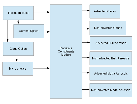
The API to be used by the radiation, optics, and microphysics parameterizations should isolate them from needing to know the source of a requested constituent distribution or property. This implies that all the logic to determine the source of constituent distributions and properties is contained in the module that implements this API and is not duplicated in all the parameterizations that need access to constituent data. Figure 6.1, “Radiative Constituents Module Dependencies” contains a schematic representation of this design.
Figure 6.1. Radiative Constituents Module Dependencies
Modules at the tails of the arrows depend on the modules at the heads of
the arrows.
The purpose of this section is to describe the radiative constituents
module (rad_constituents) which was designed to
implement this new functionality.
NOTE: The current implementation of rad_constituents does not
include the treatment of hydrometeors which comprise clouds. The
interaction of clouds and radiation remains a hardwired part of the physics
package. An implication of this for diagnostic radiative forcing
calculations is that the corresponding change in the cloud properties due
to a change in the aerosol specification will not be captured since only
the cloud representation that affects the climate is used in the radiative
transfer calculations.
The purpose of the user interface is to provide a namelist based mechanism to explicitly specify all atmospheric constituent distributions and properties that affect calculations done by the radiative transfer parameterization. All radiation calculations must be specified, that is, calculations that affect the climate as well as calculations done solely for diagnostic purposes.
In order to understand how the source of a constituent distribution is
specified it is necessary to know a few details about CAM's
infrastructure. CAM has two distinct facilities for storing
distributions, and these facilities each have private namespaces which is
why the user needs to specifiy which namespace to use when looking for a
specified constituent name. Constituent distributions fall into two
categories; either they are advected by the large scale winds (or simply
"advected") or they aren't. The constituents that are advected are stored
by CAM's infrastructure in the constituent array which is a component of
the physics state derived type. The names in the constituent array are
managed by the constituents module. Non-advected constituents are stored
in the physics buffer and names there are managed by the phys_buffer
module. To specify the source of a constituent distribution it is
sufficient, in addition to providing the distribution name, to specify
whether the constituent is advected or non-advected.
The functionality of the rad_constituents module is controlled by the
following namelist variables.
rad_climateAn array of strings indicating the set of entities that affect the climate. The format of the strings is:
rad_climate = 'entity:name:properties'
              [,'entity:name:properties'
              [,'entity:name:properties']...]
where the ':' separated terms in the strings are defined as follows:
entityAn
entitycan be either a single constituent distribution, or a group of constituents which are treated in a special way by the optics or microphysics parameterizations. Anentityis represented by a single character field which may currently take one of the following three values:AAn advected constituent distribution.
NA non-advected constituent distribution.
MA group of constituents which are treated as an aerosol mode. The mode is a mixture which has its own properties. The sources of the individual constituents that comprise the mode are given by the mode definition contained in the namelist variable
mode_defs.
nameThere are two cases, depending on the value of
entity:If
entityisM, thennameis the name of the aerosol mode and must match one of the mode names which are defined by the namelist variablemode_defs(see below).If
entityisAorN, thennameis the name by which the constituent is known to CAM's infrastructure, specifically, either theconstituentsmodule or thephys_buffermodule. Some of these names are determined via namelist input while other names may be hardcoded as part of the chemistry or aerosol parameterization which is responsible for producing them.propertiespropertiesmay be either the name of a gas phase specie that is known by the radiation parameterization, or it may be the name of a NetCDF file which is indicated by a ".nc" suffix.The optical properties of the gasses are specific to the radiation code, so it is sufficient to identify the gas properties using a name that the radiation code recognizes. The gas names recognized by both the
camrtand therrtmgradiation schemes in CAM are:H2O,O3,O2,CO2,N2O,CH4,CFC11, andCFC12.When
propertiesis specified by a NetCDF filename, the file contains the properties of either a bulk aerosol or an aerosol mode. The file is for an aerosol mode if and only if theentityisM. There will be a separate properties file for each broadband absorber (and eventually for each gas). The file will contain the necessary information to convert the distribution (plus auxiliary information such as model pressure, temperature, and humidity) to bulk layer radiative properties on each shortwave and longwave band. These bands and properties are specific to the choice of radiative transfer code.
rad_diag_1, ..., rad_diag_10The value of each of the
rad_diag_*variables is an array of strings with a format that is identical to that forrad_climatedescribed above. The constituent lists specified by these variables are for diagnostic radiation calculations only and have no impact on the climate state of the model.mode_defsmode_defsis used to define all the aerosol modes that are present in a run. Any mode that is referenced by arad_climateor arad_diag_*variable must be defined here. The value ofmode_defsis an array of strings which for each mode defined specifies the mode type, the constituents which contain the number mixing ratios for both the interstitial and cloud borne phases, and for each specie in the mode specifies which constituents contain the mass mixing ratios for both the interstitial and cloud borne phases. All modes present in the run are defined. The individual strings in the definitions have the following format:mode_defs = 'mode_name:mode_type:=', 'source_num:name_num_a:name_num_c:num_mr:+', 'source_mmr:name_mmr_a:name_mmr_c:spec_type:prop_file[:+]'[,] ['source_mmr:name_mmr_a:name_mmr_c:spec_type:prop_file][:+]['] [,...] ['mode_name:mode_type:=', 'source_num:name_num_a:name_num_c:num_mr:+', 'source_mmr:name_mmr_a:name_mmr_c:spec_type:prop_file[:+]'[,] ['source_mmr:name_mmr_a:name_mmr_c:spec_type:prop_file][:+]['] ] [,...]where the ':' separated terms in the strings are defined as follows:
mode_nameThe name of the aerosol mode being defined. The name of every aerosol mode entity in the
rad_climateorrad_diag_*variables is associated the entry inmode_defswith the matching value ofmode_name.mode_typeType of mode. Valid values are from the MAM code. The valid types for
trop_mam3areaccum,aitken, andcoarse. Additional types fortrop_mam7areprimary_carbon,fine_seasalt,fine_dust,coarse_seasalt, andcoarse_dust.=The string terminator which identifies the initial string in a mode definition.
+The string terminator which indicates that the mode definition is continued in the next string.
source_numThe source of the mode's interstitial number mixing ratio. A single character field with valid values of
AorNwhich stands for advected or non-advected constituent respectively.name_num_aThe name by which the mode's interstitial number mixing ratio is known to CAM's infrastructure.
name_num_cThe name of the mode's number mixing ratio for the cloud borne phase. Unlike the name for the interstitial phase, this name will always be known to the physics buffer module. The cloud borne phase is not advected, and thus is never registered with the constituent module.
num_mrThis is a literal term which indicates that the string is defining constituents that contain number mixing ratios. There can only be one string with the
num_mrterm in the definition of each mode.source_mmrThe source of a specie's interstitial mass mixing ratio. A single character field with valid values of
AorNwhich stands for advected or non-advected constituent respectively.name_mmr_aThe name by which a specie's interstitial mass mixing ratio is known to CAM's infrastructure.
name_mmr_cThe name of a specie's mass mixing ratio for the cloud borne phase. Unlike the name for the interstitial phase, this name will always be known to the physics buffer module. The cloud borne phase is not advected, and thus is never registered with the constituent module.
spec_typeType of specie. Valid values are from the MAM code. The valid types are
sulfate,ammonium,nitrate,p-organic,s-organic,black-c,seasalt, anddust.prop_fileName of a NetCDF file (which must have a ".nc" suffix) which contains the properties of the bulk aerosol specie that is part of the aerosol mode. The file must contain the information required by the modal optics parameterization.
For examples of the use of the namelist variables see the User's Guide.
Internally the rad_constituents module contains
lists of the gasses, bulk aerosols, and aerosol modes that contribute to
the climate and diagnostic calculations. This is essentially just a
reorganization of the data specified in
the rad_climate, rad_diag_*,
and mode_defs variables. Creating these lists (referred
to simply as gas, aerosol, and mode lists) is done by the initialization
process which begins with the rad_cnst_readnl
method, and is finished by the rad_cnst_init
method. The initialization does more that just reorganize data. It also
provides error checking to ensure that the constituents specified in the
namelist variables are known to CAM's infrastructure.
The functionality of the rad_constituents module is
provided to the application code via the following methods.
subroutine rad_cnst_readnl(nlfile)

   character(len=*), intent(in) :: nlfile  ! filepath for file containing namelist input

   namelist /rad_cnst_nl/ mode_defs,     &
                          rad_climate,   &
                          rad_diag_1,    &
                          rad_diag_2,    &
                          rad_diag_3,    &
                          rad_diag_4,    &
                          rad_diag_5,    &
                          rad_diag_6,    &
                          rad_diag_7,    &
                          rad_diag_8,    &
                          rad_diag_9,    &
                          rad_diag_10,   &
                          iceopticsfile, &
                          liqopticsfile, &
                          icecldoptics,  &
                          liqcldoptics,  &
                          oldcldoptics
rad_cnst_readnl reads the namelist
group rad_cnst_nl and parses the information in the
string arrays. The internal data structures that hold the information from
the namelist are initialized here so that the module query functions are
available at the time the register methods are called. The error checking
done during initialization is postponed to
the rad_cnst_init call since the registration
phase must occur before the availability of constituents and physics buffer
fields can be checked.
The properties files that are specified for the bulk aerosols and the
aerosol modes are managed by the phys_prop module.
The physprop_accum_unique_files subroutine is
called by rad_cnst_readnl to initialize the list
of files that that module is responsible for.
subroutine rad_cnst_init()

   ! The initialization of the gas, aerosol, and mode lists is finished by
   ! 1) reading the physprop files
   ! 2) finding the index of each constituent in the constituent or physics buffer arrays
   ! 3) finding the index of the aerosol constituents used to access its properties from the
   !    physprop module.
rad_cnst_init
calls physprop_init which reads the properties
files and finishes initializing the phys_prop
module. This module is not designed to be part of the general purpose
CAM API, but rather is designed as a utility to be used by
the rad_constituents module. All data from the
properties files should be accessed using
the rad_constituents API.
Constituents are accessed from either
the constituents or
the phys_buffer modules. Checking that the
specified constituents are available is done by this method which is called
after the registration methods. The indices used to identify constituents
in the constituents and
phys_buffer modules are saved for efficient access
during runtime. If an index is not found
then endrun is called.
interface rad_cnst_get_info
   module procedure rad_cnst_get_info
   module procedure rad_cnst_get_info_by_mode
   module procedure rad_cnst_get_info_by_mode_spec
   module procedure rad_cnst_get_info_by_spectype
end interface
subroutine rad_cnst_get_info(list_idx, gasnames, aernames, &
                             use_data_o3, ngas, naero, nmodes)

   ! Return info about gas and aerosol lists

   ! Arguments
   integer,                     intent(in)  :: list_idx    ! index of the climate or a diagnostic list
   character(len=64), optional, intent(out) :: gasnames(:)
   character(len=64), optional, intent(out) :: aernames(:)
   logical,           optional, intent(out) :: use_data_o3
   integer,           optional, intent(out) :: naero
   integer,           optional, intent(out) :: ngas
   integer,           optional, intent(out) :: nmodes
subroutine rad_cnst_get_info_by_mode(list_idx, m_idx, &
   mode_type, num_name, num_name_cw, nspec)

   ! Return info about modal aerosol lists

   ! Arguments
   integer,                     intent(in)  :: list_idx    ! index of the climate or a diagnostic list
   integer,                     intent(in)  :: m_idx       ! index of mode in the specified list
   character(len=32), optional, intent(out) :: mode_type   ! type of mode (as used in MAM code)
   character(len=32), optional, intent(out) :: num_name    ! name of interstitial number mixing ratio
   character(len=32), optional, intent(out) :: num_name_cw ! name of cloud borne number mixing ratio
   integer,           optional, intent(out) :: nspec       ! number of species in the mode
subroutine rad_cnst_get_info_by_mode_spec(list_idx, m_idx, s_idx, &
   spec_type, spec_name, spec_name_cw)

   ! Return info about modal aerosol lists

   ! Arguments
   integer,                     intent(in)  :: list_idx    ! index of the climate or a diagnostic list
   integer,                     intent(in)  :: m_idx       ! index of mode in the specified list
   integer,                     intent(in)  :: s_idx       ! index of specie in the specified mode
   character(len=32), optional, intent(out) :: spec_type   ! type of specie
   character(len=32), optional, intent(out) :: spec_name   ! name of interstitial specie
   character(len=32), optional, intent(out) :: spec_name_cw ! name of cloud borne specie
subroutine rad_cnst_get_info_by_spectype(list_idx, spectype, mode_idx, spec_idx)

   ! Return info about modes in the specified climate/diagnostics list

   ! Arguments
   integer,                     intent(in)  :: list_idx    ! index of the climate or a diagnostic list
   character(len=*),            intent(in)  :: spectype    ! species type
   integer,           optional, intent(out) :: mode_idx    ! index of a mode that contains a specie of spectype
   integer,           optional, intent(out) :: spec_idx    ! index of the species of spectype
The following sections outline how the radiative constituent interfaces are currently being used in CAM.
Note
The example code is intentionally incomplete; just pieces from the actual code have been extracted to highlight the use of the interfaces with minimal detail.
Treatment of the gas optical properties is internal to the radiation codes,
hence it is only the mixing ratio information that is passed through the
top level interfaces. The following example from the CAM4 version of
radiation_tend shows how the rad_constituents interfaces provide access
to the gas mixing ratios for the shortwave radiative calculation.
The aerosol optical properties are computed by the call to aer_rad_props_sw.
subroutine radiation_tend(...)

    use rad_constituents, only: rad_cnst_get_gas

    real(r8), pointer :: sp_hum(:,:)         ! specific humidity
    real(r8), pointer :: o3(:,:)             ! Ozone mass mixing ratio
    real(r8), pointer :: o2(:,:)             ! Oxygen mass mixing ratio
    real(r8),         :: o2_col(pcols)       ! column oxygen mmr
    real(r8), pointer :: co2(:,:)            ! co2 mass mixing ratio
    real(r8),         :: co2_col_mean(pcols) ! co2 column mean mmr

    ! Get specific humidity
    call rad_cnst_get_gas(0,'H2O', state, pbuf, sp_hum)

    ! Get ozone mass mixing ratio.
    call rad_cnst_get_gas(0,'O3',  state, pbuf, o3)

    ! Get CO2 mass mixing ratio and compute column mean values
    call rad_cnst_get_gas(0,'CO2', state, pbuf, co2)
    call calc_col_mean(state, co2, co2_col_mean)

    ! Get Oxygen mass mixing ratio and compute column mean values
    call rad_cnst_get_gas(0,'O2', state, pbuf, o2)
    call calc_col_mean(state, o2, o2_col)

    ! Get aerosol radiative properties.
    call aer_rad_props_sw(0, state, pbuf, nnite, idxnite, &
         aer_tau, aer_tau_w, aer_tau_w_g, aer_tau_w_f)

    call radcswmx(..., sp_hum, o3, o2_col, co2_col_mean, ..., &
                 aer_tau, aer_tau_w, aer_tau_w_g, aer_tau_w_f, ...)
The first argument to both rad_cnst_get_gas and aer_rad_props_sw
determines whether the climate list or one of the diagnostic lists is used
to specify the constituents. Here that argument is hardcoded to 0 which
means use the climate list. The CAM4 radiation code doesn't support
diagnostic radiative forcing calculations.
The gas name given as the second argument must be a name recognized by the
radiation code. These names are contained in the radconstants module.
The version of radiation_tend used by CAM5 (RRTMG) is very similar, the
main difference being that the first argument to rad_cnst_get_gas and
aer_rad_props_sw is a variable that can be set to use any of the climate
or diagnostic lists in the radiative transfer calculation.
The bulk aerosol optical properties are computed outside the radiation code and are passed to it via the argument list. The optical properties of the individual bulk aerosol species are "externally mixed" by which we mean that the properties of the whole are treated as the sum of the parts. Hence the calculation of the bulk aerosol properties are done in a loop over the list of bulk aerosol species and the properties of the whole are accumulated as the sum over the properties of the individual species.
The computation of the aerosol optical layer properties is done by routines
in the aer_rad_props module. The following example is from the routine
for the shortwave calculation.
subroutine aer_rad_props_sw(list_idx, state, pbuf, nnite, idxnite, &
                            tau, tau_w, tau_w_g, tau_w_f)

   use rad_constituents, only: rad_cnst_get_info, rad_cnst_get_aer_mmr, &
                               rad_cnst_get_aer_props

   real(r8), pointer :: aermmr(:,:)    ! mass mixing ratio of aerosols

   ! compute mixing ratio to mass conversion
   mmr_to_mass(:,:) = rga * state%pdeldry(:,:)

   ! initialize optical property output
   tau     (:,:,:) = 0._r8
   tau_w   (:,:,:) = 0._r8
   tau_w_g (:,:,:) = 0._r8
   tau_w_f (:,:,:) = 0._r8

   ! get number of bulk aerosols in current list
   call rad_cnst_get_info(list_idx, naero=numaerosols)

   ! Contributions from bulk aerosols.
   do aer_idx = 1, numaerosols

      ! get bulk aerosol mass mixing ratio
      call rad_cnst_get_aer_mmr(list_idx, aer_idx, state, pbuf, aermmr)
      aermass(:,:) = aermmr(:,:) * mmr_to_mass(:,:)

      ! get optics type
      call rad_cnst_get_aer_props(list_idx, aer_idx, opticstype=opticstype)

      select case (trim(opticstype))
      case('hygro','hygroscopic','hygroscopi')
         ! get optical properties for hygroscopic aerosols
         call rad_cnst_get_aer_props(list_idx, aer_idx, sw_hygro_ext=h_ext, &
                                     sw_hygro_ssa=h_ssa, sw_hygro_asm=h_asm)
         call get_hygro_rad_props(ncol, krh, wrh, aermass, h_ext, h_ssa, h_asm, &
                                  ta, tw, twg, twf)

      case('nonhygro','insoluble ')
         ! get optical properties for non-hygroscopic aerosols
         call rad_cnst_get_aer_props(list_idx, aer_idx, sw_nonhygro_ext=n_ext, &
                                     sw_nonhygro_ssa=n_ssa, sw_nonhygro_asm=n_asm)
         call get_nonhygro_rad_props(ncol, aermass, n_ext, n_ssa, n_asm, &
                                     ta, tw, twg, twf)

      case('volcanic')
         ! get optical properties for volcanic aerosols
         call rad_cnst_get_aer_props(list_idx, aer_idx, sw_nonhygro_ext=n_ext, &
                              sw_nonhygro_scat=n_scat, sw_nonhygro_ascat=n_ascat)
         call get_volcanic_rad_props(ncol, aermass, n_ext, n_scat, n_ascat, &
                                     ta, tw, twg, twf)

      case('volcanic_radius')
         ! get optical properties for volcanic aerosols
         call rad_cnst_get_aer_props(list_idx, aer_idx, r_sw_ext=r_ext, &
                            r_sw_scat=r_scat, r_sw_ascat=r_ascat, mu=r_mu)
         call get_volcanic_radius_rad_props(lchnk, ncol, aermass, pbuf, r_ext, &
                                        r_scat, r_ascat, r_mu, ta, tw, twg, twf)

      end select

      tau    (:,:,:) = tau    (:,:,:) + ta (:,:,:)
      tau_w  (:,:,:) = tau_w  (:,:,:) + tw (:,:,:)
      tau_w_g(:,:,:) = tau_w_g(:,:,:) + twg(:,:,:)
      tau_w_f(:,:,:) = tau_w_f(:,:,:) + twf(:,:,:)

   enddo
The number of bulk aerosol species is returned by the first call to
rad_cnst_get_info. The first argument to that
call, list_idx, specifies whether the aerosols are in
the climate list (index 0) or one of the diagnostic lists.
Inside the loop over the aerosol species the first call to
rad_cnst_get_aer_mmr returns a pointer to the mixing ratio for
the aer_idx specie in the list. The mixing ratio is
then converted to a mass.
Next the call to rad_cnst_get_aer_props returns the optics type. This
information comes from the properties file that is associated with each
bulk aerosol specie. It's value is used in the case selector to determine
which method to use for the optics properties calculations.
Once inside the case selector the rad_cnst_get_aer_props method is called
again and returns the specific properties required by the method that is
used for the optics calculation. Again these properties come from the
associated properties dataset.
The optical properties of an aerosol mode are computed using properties of the species that comprise the mode along with properties that pertain to the mixture of the species contained in the mode. The optical properties of modes are externally mixed (summed) to give the total contribution to the aerosol optical properties from the modes.
The calculation of the optical properties due to aerosol modes is done in
the modal_aer_opt module. The following example is from the routine for
the shortwave calculation.
subroutine modal_aero_sw(list_idx, state, pbuf, nnite, idxnite, &
                         tauxar, wa, ga, fa)

   use rad_constituents, only: rad_cnst_get_info, rad_cnst_get_aer_mmr, &
                             rad_cnst_get_aer_props, rad_cnst_get_mode_props

   ! initialize output variables
   tauxar(:ncol,:,:) = 0._r8
   wa(:ncol,:,:)     = 0._r8
   ga(:ncol,:,:)     = 0._r8
   fa(:ncol,:,:)     = 0._r8

   ! get number of aerosol modes
   call rad_cnst_get_info(list_idx, nmodes=nmodes)

   do m = 1, nmodes

      ! get mode properties
      call rad_cnst_get_mode_props(list_idx, m, sigmag=sigma_logr_aer, refrtabsw=refrtabsw , &
                          refitabsw=refitabsw, extpsw=extpsw, abspsw=abspsw, asmpsw=asmpsw)

      ! get number of species in mode
      call rad_cnst_get_info(list_idx, m, nspec=nspec)

      do isw = 1, nswbands

         do k = 1, pver

            ! aerosol species loop
            do l = 1, nspec
               call rad_cnst_get_aer_mmr(list_idx, m, l, 'a', state, pbuf, specmmr)
               call rad_cnst_get_aer_props(list_idx, m, l, density_aer=specdens, &
                                    refindex_aer_sw=specrefindex, spectype=spectype)

            end do ! species loop

            ! compute dopaer, palb, pasm

            do i=1,ncol
               tauxar(i,k,isw) = tauxar(i,k,isw) + dopaer(i)
               wa(i,k,isw)     = wa(i,k,isw)     + dopaer(i)*palb(i)
               ga(i,k,isw)     = ga(i,k,isw)     + dopaer(i)*palb(i)*pasm(i)
               fa(i,k,isw)     = fa(i,k,isw)     + dopaer(i)*palb(i)*pasm(i)*pasm(i)
            end do

         end do ! pver

      end do ! sw bands

   end do ! nmodes
The first call to rad_cnst_get_info returns the number of modes in the
list specified by list_idx.
The call to rad_cnst_get_mode_props inside the loop over modes is to get
properties that are specific to the mode. The call to rad_cnst_get_info
returns the number of species in mode m. Note that
rad_cnst_get_info is a generic interface. In the first call with only
one required argument it returns information that's relevent to a given
list, while in the second call with two required arguments it's returning
information relevent to a mode in the list.
Inside the loop over species the calls to rad_cnst_get_aer_mmr and
rad_cnst_get_aer_props are returning mixing ratios and properties for
specie l in mode m. Again note the
overloading of these generic interfaces. In the previous section on bulk
aerosol optical properties these routines were called with two required
arguments and returned properties of bulk aerosols. Here
rad_cnst_get_aer_props is called with three required arguments and is
returning properties of species comprising an aerosol mode.
rad_cnst_get_aer_mmr is called with four required arguments; in addition
to mode and specie indices, it is also necessary to specify whether the
mixing ratio is for the interstitial ('a'), or the cloud
borne ('c') phase.
The CAM subcolumn infrastructure provides the ability to create fields with several elements within a single grid column. Different methods for generating and averaging subcolumn fields are called subcolumn schemes and are designated with the 'subcol_scheme' namelist variable. This chapter describes how to define a new subcolumn scheme and how to create and use subcolumn fields in a physics parameterization.
In order to implement a new scheme, you need to follow these steps:
Implement a subcolumn scheme in a separate module (subcol_<scheme>.F90). This scheme may use data from a physics parameteriztion but not from an interface module (<param>_intr.F90). It may also use data from ppgrid, physconst, and physics_buffer.
Implement a subcol_register_<scheme> subroutine to register any scheme-specific fields. Any pbuf_add_field calls need to go here, however, pbuf fields are normally only used when the data is also used by another module so most pbuf_add_field calls will be in a parameterization module. See the restart routines below to see how other module data may be saved. This step is optional.
Implement a subcol_readnl_<scheme> subroutine to read in the namelist variables for this scheme's namelist. This step is optional.
Implement a subcol_init_<scheme> function to initialize any scheme- specific variables or fields. This is also a good time to call pbuf_get_index to store any pbuf indices needed later. This step is optional.
Implement a subcol_gen_<scheme> function to generate the appropriate subcol fields based on the existing GBA fields and other scheme data.
Implement a subcol_field_avg_<scheme> function to average subcol fields back into the appropriate GBA fields.
Implement a subcol_ptend_avg_<scheme> function to average the subcolumn ptend to a grid ptend This step is optional
Add necessary cases in the master subcol module (subcol.F90)
Add a case for your scheme name in subcol_register and optionally call your subcol_<scheme> registration function. subcol_register is called at registration time in phys_register.
Add a case for your scheme name in subcol_init and optionally call your subcol_<scheme> initialization function. subcol_init is called at initialization time in phys_init.
Add a case for your scheme name in subcol_gen and call your subcol_<scheme> subcol generator. subcol_gen is called in tphysbc although it can also be called by other parameterizations for special-purpose subcolumn use.
Add a case for your scheme name in subcol_field_avg and call your subcol_<scheme> field-averaging function.
Add a case for your scheme name in subcol_ptend_avg and optionally call your subcol_<scheme> ptend-averaging function.
NB: New schemes should be implemented in a separate file which is used by this module (and thus may not 'use' any subcol module variable, function, or subroutine).
Most subcolumn schemes contain information which must be stored acros time steps. This information can be stored as module variables. However, in cases where there is an interaction between the subcolumn scheme and other CAM physics code (e.g., subcolumns populated according to a PDF generated by a physics parameterization), this information can also be stored in subcolumn fields (see Section 6.2.2, “Subcolumn fields”).
To create a subcolumn field, call pbuf_add_field in a physics registration subroutine. By using the optional sixth argument, grid_types_flag. This flag can be set to create a grid-average field, a subcolumn field, or both.
NB: If a subcolumn generator changes the number of subcolumns in a grid column. subcolumn fields which persist across time steps need to be reformed.
Table of Contents
The CAM grid infrastructure provides an object which holds information about one CAM grid (e.g., a dycore grid) being used in the current run. The grid object contains all information about the grid's axes, the grid's lon/lat points, and its layout relative to NetCDF file order (e.g., its decomposition).
CAM grid objects are distributed objects; The object on each task only holds information on the grid's task-local points. CAM maintains an array of grids which are referenced through a handle
A horizontal coordinate is an object which describes the horizontal coordinate for one or more grids. For structured grids, these are simply longitude ('lon') and latitude ('lat'). For unstructured grids, which have 'columns' defined in longitude and latitude, these coordinates are defined in terms of the grid's column dimension. The horiz_coord_t type contains the following elements:
name- name
coordinate name (e.g., 'lon', 'lat_s')
- dimname: type: character(len=max_hcoordname_len)
dimension name. This is used for unstructured grids where the dimension name (e.g., 'ncol') is the coordinate variable. If dimname is blank, then name is used as a coordinate variable.
- dimsize = 0: type: integer
size of dimension
- long_name = '': type: character(len=max_chars)
'long_name' attribute
- units = '': type: character(len=max_chars)
'units' attribute
- values(:) => null(): type: real(r8), pointer
dim values (local if map)
- map(:) => null(): type: integer(iMap), pointer
map (dof) for dist. coord
- latitude: type: logical
.false. means longitude
[Craig et al.[2012]] Craig, Anthony P., Mariana Vertenstein, and Robert Jacob. A new flexible coupler for earth system modeling developed for CCSM4 and CESM1 , The International Journal of High Performance Computing Applications, (1), 31-42, doi:10.1177/1094342011428141 , 2012.
[Kalnay et al.[1989]] Kalnay, E., M. Kanamitsu, J. Pfaendtner, J. Sela, M. Suarez, J. Stackpole, J. Tuccillo, L. Umscheid, and D. Williamson. Rules for Interchange of Physics Parameterizations , Bulletin American Meteorological Society, (6), 620-622, 1989.
[Worley et al. [2005]] Worley, Patrick H., and John B. Drake. Performance Portability in the Physical Parameterizations of the Community Atmospheric Model , The International Journal of High Performance Computing Applications, (3), 187-201, doi:10.1177/1094342005056095 , 2005.