9 The cpl6 main

This section provides guidance to understanding the cpl6 main program which coordinates the transfer of data between components in CCSM3.

9.1 Variable Naming Conventions

A variable naming convention has been adopted to help organize and identify the literally hundreds of state and flux fields managed by the Coupler. Understanding this naming convention will aid understanding the main code and pseudo-code below.

9.1.1 State Variables

Model state variables are denoted Sx, where x denotes the corresponding component model:

9.1.2 Flux Fields

Input flux means fluxes given by the Coupler to a model. Output flux means fluxes computed within a model and given to the Coupler. All input fluxes for one model were either computed by the Coupler or were the output flux of another model. In general, a given flux field between any two component models may have been computed in one of three places: within either of the two models or within the Coupler.

One function of the Coupler is to gather, merge, sum, and/or time-average the various component flux fields from various sources and form a set of complete input fluxes for each component model. This gathering and merging process will generally involve mapping flux fields between various model grids and combining like fields from several grids onto one grid. A summation might be required, e.g., net heat flux = solar + latent + sensible + longwave. Also, for some flux fields the Coupler might be required to form time-averaged quantities. Thus component fluxes are mapped, merged, summed, and/or time-averaged by the Coupler in order to form complete input fluxes for the models.

Flux fields are denoted Fxyz, where xy denotes the two model between which a quantity is being fluxed, and z denotes the model which computed the flux (i.e. it is an output flux of model z).

Component fluxes that are gathered, merged, summed, and/or time-averaged to form the complete input fluxes are:

9.1.3 Domain Maps

Mapping between domains is implemented by matrix multiplies. Generally there are different maps for state fields vs. flux fields, as state fields maps are generally smoother (e.g. bilinear) whereas flux field maps must be conservative (e.g.. area averaging, aka Riemann sum integrals). In the case of mapping between identical domains, the map would be the identity map. The necessary mapping matrices are:

9.1.4 Bundles and Contracts

The Coupler declares several instances of the BUNDLE and CONTRACT datatypes and they also follow a naming convention. Bundles have names similar to the map's but with an extra postfix to identify which grid the data is on. For example:

The names of Contracts also contain a direction but, since the BUNDLE in the CONTRACT contains both State and Flux data, an ``X'' is used in the name.

9.2 Scientific Assumptions in main

The code of the cpl6 main fixes many of the assumptions and scientific requirements of CCSM3. This section describes which assumptions/requirements have been ``hard-coded'' into CCSM3's coupler. However, because of the modular structure of the cpl6 code, it is straightforward to remove most of these assumptions and allow alternate configurations of CCSM3 components.

9.2.1 Number of Components

Since the river model runs on a different grid, the Coupler establishes a separate contract for the one-way exchange of information from the river model to the Coupler and the river model is treated as a sixth component. But in the MPI view of CCSM, the land and river models are on the same processors and share the same MPI communicator.

9.2.2 Number of Grids

The Coupler main assumes there are only 3 different grids however the size and type of each grid may change. The atmosphere and land models are assumed to share the same grid and the ocean and sea ice models are also assumed to share the same grid (but different from the atmosphere-land). The river model's grid is the third grid in the CCSM3 Coupler.

9.2.3 Time Integration and Coordination

9.2.4 Data Pathways through the Coupler

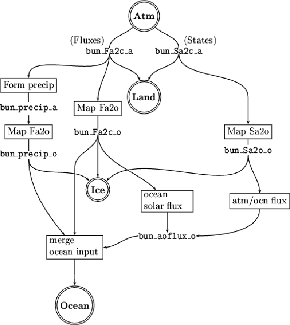
The Coupler code allows only certain data pathways between models. We define a ``pathway'' as the sequence of operations performed on data sent from a component model to the Coupler on it's way to another model. An example is shown in Figure 2. Figure 2 shows what happens to the BUNDLE

**Figure 2:** The pathway of data from the atmosphere model through the coupler. Note that not all operations are shown
$\begin{figure}\centering\epsfbox{figs/datapath.eps}\end{figure}$

Some pathways are not implemented in the current release of the Coupler. There is no path directly from the land model to the ocean model (although there is a path from the river model to the ocean model.) Pathways which do exist have only certain operations. For example in the path between the ice and the ocean model, there is no mapping because it is assumed that the ice and ocean models are on the same grid (Section 9.2.2).

9.3 Main Program Detail

To understand the details of the Coupler's functionality, it is useful to have a basic understanding of the Coupler main's source code. To that end, pseudo-code for main is shown below. If one wishes to modify the Coupler source code, it is strongly recommended that one first study this section in conjunction with studying the source code file, main.F90. This should provide a good overview of how the Coupler works; a necessary pre-requisite for successful code modification.

9.3.1 Psuedocode for main

In the pseudocode below, code from the Coupler is in typewriter font. Comments about the code are in italics and summaries representing sections of code are in [ALL CAPS].

PROGRAM main [INITIALIZE TIMERS] Initialize MPI and get local MPI communicator call cpl_interface_init(cpl_fields_cplname,local_comm) Read the Coupler namelist call cpl_control_readNList() Get simulation start date call restart_readDate(cDate) Initialize the Coupler infobuffers in each Contract call cpl_infobuf_init(con_Xa2c%infobuf) [INITIALIZE OTHER INFOBUFFERS] Initialize receiving Contract with atmosphere call cpl_interface_contractInit(con_Xa2c,cpl_fields_cplname, & cpl_fields_atmname,cpl_fields_a2c_fields,bunname="Xa2c_a", & decomp=cpl_control_decomp_a) Initialize sending Contract with atmosphere call cpl_interface_contractInit(con_Xc2a,cpl_fields_cplname, & cpl_fields_atmname,cpl_fields_c2a_fields,bunname="Xc2a_a", & decomp=cpl_control_decomp_a) dom_a = con_Xa2c%domain Make sure domains are identical con_Xc2a%domain = dom_a [INITIALIZE CONTRACTS WITH ICE AND OCEAN MODEL] [INITIALIZE SPECIAL DOMAIN CONTRACT WITH LAND MODEL. DETERMINE IF COUPLER SHOULD SEND LAND DOMAIN.] Initialize inter-domain area fractions call frac_init(map_Fo2a,dom_a,dom_i,dom_l,dom_o) [IF REQUESTED, DETERMINE LAND DOMAIN AND SEND TO LAND MODEL] [INITIALIZE CONTRACTS WITH LAND AND RIVER MODEL] [CHECK THAT LAND AND ATMOSPHERE DOMAINS ARE CONSISTENT] [CHECK THAT ICE AND OCEAN DOMAINS ARE CONSISTENT] call data_bundleInit() Initialize Coupler bundles call data_mapInit() Initialize Coupler maps for interpolation call history_avbundleInit() Initialize history buffers [SET VALUES FOR INITIAL INFOBUFFER] Send infobuffer to atmosphere call cpl_interface_infobufSend(cpl_fields_atmname, con_Xc2a%infobuf%ibuf,con_Xc2a%infobuf%rbuf) [SEND INFOBUFFERS TO OCEAN, ICE, LAND AND RIVER MODELS] [VERIFY ACCEPTABLE COUPLING INTERVALS.] [CHECK FOR DEAD COMPONENTS.] date = shr_date_initCDate(cDate,ncpl_a) Initalize model start date call cpl_control_init(date) and control flags call cpl_control_update(date) [RESET BUNDLE DOMAINS AREAS TO MAP FILES AREAS] Receive initial condition data from atmosphere call cpl_interface_contractRecv(cpl_fields_atmname,con_Xa2c) Multiply received data by normalized area call cpl_bundle_mult(con_Xa2c%bundle,bun_areafact_a,'comp2cpl', & bunlist=cpl_fields_a2c_fluxes) [RECEIVE INITIAL DATA FROM ICE, LAND, RIVER AND OCEAN MODELS] call restart_read(date) Read restart [PROCESS (SPLIT INTO BUNDLES AND MAP) INITIAL CONDITION DATA] [IF REQUESTED, SEND ALBEDO TO ATMOSPHERE AND GET NEW INITIAL DATA] DO WHILE ( .not. cpl_control_stopNow ) Main integration loop DO n=0,ncpl_a Loop over number of atmosphere communications per day Send message to ocean if(mod(n-1,ncpl_a/ncpl_o) == 0 ) then If time to talk to ocean if (.not. cpl_control_lagOcn) then multiply sent data by normalized area call cpl_bundle_mult(con_Xc2o%bundle,bun_areafact_o, & 'cpl2comp',bunlist=cpl_fields_c2o_fluxes) Send the data call cpl_interface_contractSend(cpl_fields_ocnname,con_Xc2o) multiply sent data by inverse of normalized area call cpl_bundle_mult(con_Xc2o%bundle,bun_areafact_o, & 'comp2cpl', bunlist=cpl_fields_c2o_fluxes) endif call cpl_bundle_zero(bun_Xc2oPSUM_o) zero out the partial sum endif if (mod(n-1,ncpl_a/ncpl_l) == 0 ) then [SEND DATA TO LAND MODEL] Map atmosphere states (from initial receive or previous step) to ocean grid call cpl_map_bun(bun_Sa2c_a,bun_Sa2c_o,map_Sa2o,mvector=a2ovector) Map atmosphere fluxes to ocean grid) call cpl_map_bun(bun_Fa2c_a,bun_Fa2c_o,map_Fa2o,mvector=a2ovector) [IF REQUESTED, FORCE BALANCE THE FRESH WATER FLUX] Correct the a2o vector mapping near north pole call cpl_map_npfix(bun_Sa2c_a,bun_Sa2c_o,'Sa_u','Sa_v') [SEND DATA TO ICE MODEL] Compute net solar flux into ocean. call flux_solar(bun_Fa2c_o, bun_oalbedo_o, bun_aoflux_o ) call merge_ocn() merge ocean inputs Form time average of ocean inputs call cpl_bundle_accum(bun_Xc2oSNAP_o,outbun=bun_Xc2oPSUM_o) [DO DIAGNOSTICS] call flux_albo(date,bun_oalbedo_o) Compute ocean albedos. (Sec. 16.3.3) Compute atmosphere/ocean fluxes. (Sec. 16.2) call flux_atmOcn(con_Xo2c%bundle,bun_Sa2c_o,cpl_control_dead_ao, bun_aoflux_o ) if (mod(n-1,ncpl_a/ncpl_i) == 0 ) then [RECEIVE DATA FROM ICE MODEL] If requested, add diurnal cycle to ice albedo. (Sec. 16.3.2) call flux_albi(date,con_Xi2c%bundle) Split received ice data into states and fluxes call cpl_bundle_split(con_Xi2c%bundle,bun_Si2c_i,bun_Fi2c_i) Map ice and ocean states to atmosphere grid call cpl_map_bun(bun_Si2c_i,bun_Si2c_a,map_So2a, & bun_frac_i,'ifrac',bun_frac_a,'ifrac',oi2avector) call cpl_map_bun(bun_So2c_o,bun_So2c_a,map_So2a, & bun_frac_o,'afrac',bun_frac_a,'ofrac',oi2avector) [MAP ICE AND OCEAN FLUXES TO ATMOSPHERE GRID] if (mod(n-1,ncpl_a/ncpl_l) == 0 ) then [RECEIVE DATA FROM LAND MODEL] if (mod(n,ncpl_a/ncpl_r) == 0 ) then [RECEIVE DATA FROM RIVER MODEL] call merge_atm(fix_So2c_a) Merge atmosphere state and flux fields if (mod(n-1,ncpl_a/ncpl_a) == 0 ) then [SEND DATA TO ATMOSPHERE MODEL] Map river model data to ocean grid call cpl_map_bun(con_Xr2c%bundle,bun_Xr2c_o,map_Xr2o,mvector=r2ovector) call history_write(date) Create and/or update history files call history_avwrite(date) if (mod(n,ncpl_a/ncpl_o) == 0 ) then [RECEIVE DATA FROM OCEAN] if (mod(n-1,ncpl_a/ncpl_a) == 0 ) then [RECEIVE DATA FROM ATMOSPHERE] call shr_date_adv1step(date) Advance date and update control flags call shr_date_getCDate(date,cDate,sec) call shr_date_getYMD(date,year,month,day,sec) call cpl_control_update(date) END DO call timeCheck(date,.false.,.true. ) Verify time coordination END DO WHILE End of main integration loop call history_avwrite(date) Write last history file Send final message to atmosphere call cpl_interface_contractSend(cpl_fields_atmname,con_Xc2a) [SEND FINAL MESSAGE TO ICE, LAND AND OCEAN MODELS] call cpl_interface_finalize(cpl_fields_cplname) Disconnect from MPI STOP/END OF PROGRAM

9.3.2 A Data Pathway in Detail

With the pseudocode, the *_field definitions in cpl_fields_mod.F90, and the BUNDLE initializations in data_mod.F90, one can determine how the attribute names in a BUNDLE are used to route data through pathways. Consider the incoming atmosphere bundle shown in Fig. 2. The BUNDLE in Con_Xa2c%bundle is initialized using the cpl_fields_a2c_fields string while bun_Sa2c_a is initialized with the cpl_fields_a2c_states substring and bun_Fa2c_a is initialized with the cpl_fields_a2c_fluxes substring. The call to cpl_bundle_split copies the data in Con_Xa2c%bundle into bun_Sa2c_a or bun_Fa2c_a according to the matching attribute names. Since, by construction, *_fields is the union of *_states and *_fluxes, the split is exact.

Attribute name matching is also used the move data through the Fa2o mapping call shown in Fig. 2. This call will automatically map all the fields in bun_Fa2c_a which have the same names as the fields in the output BUNDLE bun_Fa2c_o. Since bun_Fa2c_o is also initialized with cpl_fields_a2c_fluxes (in data_mod.F90), the entire contents of bun_Fa2c_a are mapped to the ocean grid.

Finally, attribute name matching is used to ``gather'' data for passing out to a component model using cpl_bundle_gather. Note that this does not mean ``gather'' in the MPI sense of gathering distributed data to a single processor. It means gathering data from several BUNDLES with the same attribute name into one outgoing BUNDLE. For example, cpl_fields_a2c_states and cpl_fields_c2i_states both contain an attribute called ``Sa_u''. Since the same name appears in both the Con_Xa2c%bundle, bun_Sa2c_o, and Con_Xc2i%bundle, this ensures that the data contained in the ``Sa_u'' slot in the Con_Xa2c%bundle, the atmosphere's zonal wind field, will be mapped to the ice/ocean grid with the correct mapping and sent to the ice model.

9 The cpl6 `main`

9.1 Variable Naming Conventions

9.1.1 State Variables

9.1.2 Flux Fields

9.1.3 Domain Maps

9.1.4 Bundles and Contracts

9.2 Scientific Assumptions in `main`

9.2.1 Number of Components

9.2.2 Number of Grids

9.2.3 Time Integration and Coordination

9.2.4 Data Pathways through the Coupler

9.3 Main Program Detail

9.3.1 Psuedocode for `main`

9.3.2 A Data Pathway in Detail

9.1 Variable Naming Conventions

9.2 Scientific Assumptions in main

9.2.2 Number of Grids

9.2.4 Data Pathways through the Coupler

9.2 Scientific Assumptions in `main`