
Research Highlights from the Polar Climate Working Group
- Inter-annual to multi-decadal Arctic sea ice extent trends in a warming world.
- Sea ice reversibility.
- Improved sea ice shortwave physics in CCSM4.
- 21st-Century Arctic Climate Change in CCSM4.
- Arctic inversion strength in climate models.
- A Characterization of the Present-Day Arctic Atmosphere in CCSM4.
- Abrupt onset of the Little Ice Age triggered by volcanism and sustained by sea-ice/ocean feedbacks.
- Coupling between Arctic feedbacks and changes in poleward energy transport.
- Late 20th century simulation of Arctic sea ice and ocean properties in the CCSM4.
- Antarctic Sea Ice Climatology and Variability.
A climate model (CCSM4) is used to investigate the influence of anthropogenic forcing on late 20th century and early 21st century Arctic sea ice extent trends. On all timescales examined (2-50+ years), the most extreme negative observed late 20th century trends cannot be explained by modeled natural variability alone. Modeled late 20th century ice extent loss also cannot be explained by natural causes alone, but the six available CCSM4 ensemble members exhibit a large spread in their late 20th century ice extent loss. Comparing trends from the CCSM4 ensemble to observed trends suggests that internal variability explains approximately half of the observed 1979-2005 September Arctic sea ice extent loss. In a warming world, CCSM4 shows that multi-decadal negative trends increase in frequency and magnitude, and that trend variability on 2-10 year timescales increases (Figure 1). Furthermore, when internal variability counteracts anthropogenic forcing, positive trends on 2-20 year timescales occur until the middle of the 21st century.
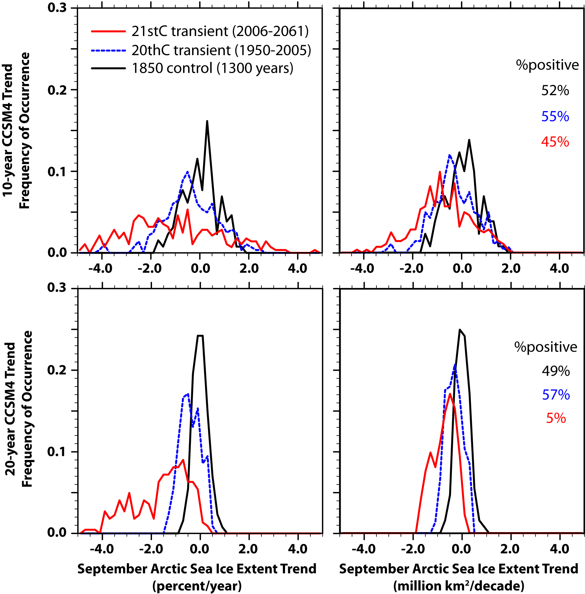
Figure 1. Modeled distributions of 10 and 20 year Arctic sea ice extent trends. Figure adapted from Kay et al. (2011) Figure 3 and supplementary material.
We test sea ice reversibility within a state‐of‐the‐art atmosphere–ocean global climate model (CCSM3) by increasing atmospheric carbon dioxide until the Arctic Ocean becomes ice‐free throughout the year and subsequently decreasing it until the initial ice cover returns. Evidence for irreversibility in the form of hysteresis outside the envelope of natural variability is explored for the loss of summer and winter ice in both hemispheres. We find no evidence of irreversibility or multiple ice‐cover states over the full range of simulated sea ice conditions between the modern climate and that with an annually ice‐free Arctic Ocean. Summer sea ice area recovers as hemispheric temperature cools along a trajectory that is indistinguishable from the trajectory of summer sea ice loss, while the recovery of winter ice area appears to be slowed due to the long response times of the ocean near the modern winter ice edge. These findings serve as evidence against the existence of threshold (or 'tipping point') behavior in the summer or winter ice cover in either hemisphere.
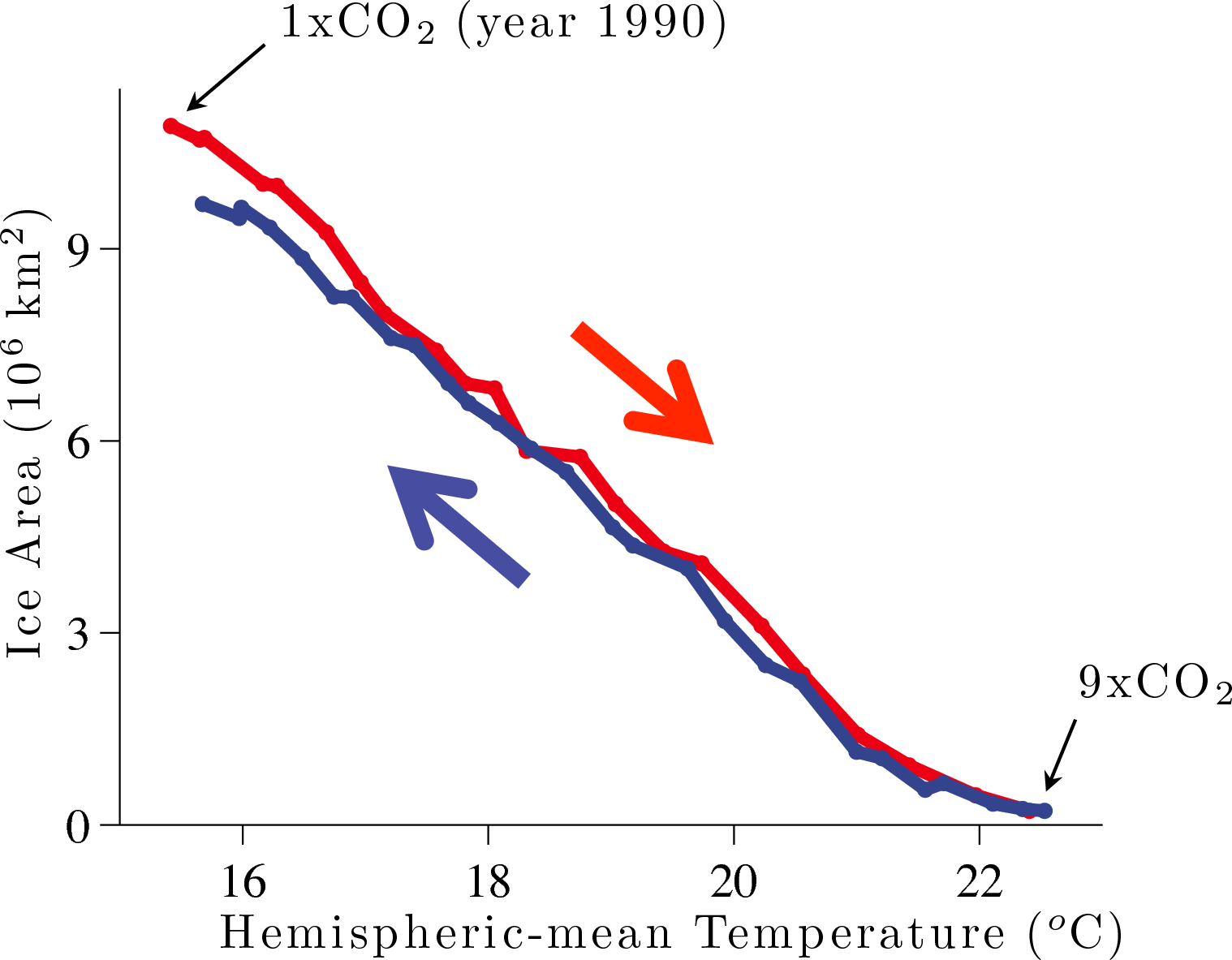
Figure 1: Northern Hemisphere sea ice area and hemispheric-mean temperature, both plotted as 10-year means, when CO2 is increased and then decreased in CCSM3. The simulation shows no evidence of irreversible sea ice loss. Adapted from Armour et al. 2011, Figure 2.
In CCSM4 the most notable improvements to the sea ice model are the incorporation of a new shortwave radiative transfer scheme and the capabilities that this enables. This scheme uses inherent optical properties to define scattering and absorption characteristics of snow, ice and included shortwave absorbers and explicitly allows for melt ponds and aerosols. The deposition and cycling of aerosols in sea ice is now included and a new parameterization derives ponded water from the surface meltwater flux. Taken together, this provides a more sophisticated, accurate, and complete treatment of sea ice radiative transfer. In preindustrial simulations, the radiative impact of ponds and aerosols on Arctic sea ice is 1.1 W/m2 annually, with aerosols accounting for up to 8 W/m2 enhanced June shortwave absorption in the Barents/Kara Seas, and with ponds accounting for over 10 W/m2 in shelf regions in July. In 2XCO2 simulations with the same aerosol deposition, ponds have a larger effect whereas aerosol effects are reduced, thereby modifying the surface albedo feedback. While the direct forcing is modest, because aerosols and ponds influence the albedo, the response is amplified. In simulations with no ponds or aerosols in sea ice, the Arctic ice is over a meter thicker and retains more summer ice cover. Diagnosis of a 20th century simulation (FIGURE) indicates an increased radiative forcing from aerosols and melt ponds, which could play a role in 20th century Arctic sea ice reductions. In contrast, ponds and aerosol deposition have little effect on Antarctic sea ice for all climates considered.
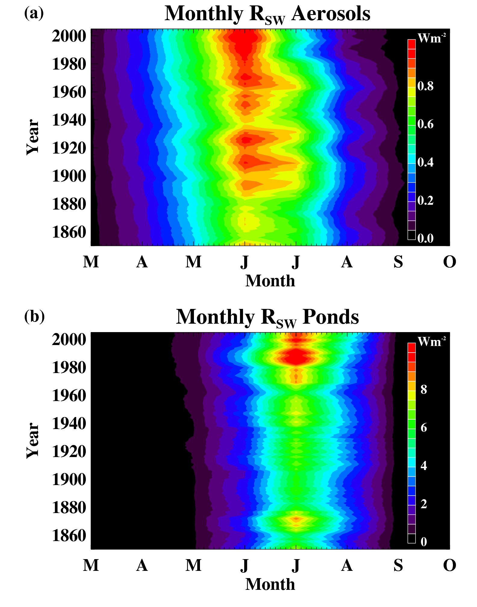
Figure 1: The Arctic monthly averaged shortwave radiative forcing in W m-2 associated with (a) aerosols and (b) melt ponds in sea ice for the 20th century simulation. Note the different color scale for the two panels.
Vavrus, S. J., M. M. Holland, A. Jahn, D. A. Bailey, and B. A. Blazey, 2011: 21st-Century Arctic Climate Change in CCSM4. J. Climate, in revision.
We summarize the 21st-century Arctic climate simulated by the latest version of NCAR’s Community Climate System Model, CCSM4. Under a strong radiative forcing scenario, the model simulates a much warmer, wetter, cloudier, and stormier Arctic climate with considerably less sea ice and a fresher Arctic Ocean. The high correlation among the variables comprising these changes---temperature, precipitation, cloudiness, sea level pressure (SLP), and ice concentration---suggests that their close coupling collectively represents a fingerprint of Arctic climate change. Although the projected changes in CCSM4 are generally consistent with those in other GCMs, we identify several noteworthy features. Despite more global warming in CCSM4, Arctic changes are generally less than under comparable greenhouse forcing in CCSM3, as represented by Arctic amplification (16% weaker) and the date of a seasonally ice-free Arctic Ocean (20 years later). Autumn is the season of most pronounced Arctic climate change among all the primary variables. The changes are very similar across the five ensemble members, although SLP displays the largest internal variability. The SLP response exhibits a significant trend toward stronger extreme Arctic cyclones, implying greater wave activity that would promote coastal erosion. Based on a commonly used definition of the Arctic (the area encompassing the 10oC July air temperature isotherm), the region shrinks by about 40% during the 21st century, in conjunction with a nearly 10 K warming trend poleward of 70oN. Despite this pronounced long-term warming, CCSM4 simulates a hiatus in the secular Arctic climate trends during a decade-long stretch in the 2040s and to a lesser extent in the 2090s. These pauses occur despite averaging over five ensemble members and are remarkable because they happen under the most extreme greenhouse-forcing scenario and in the most climatically sensitive region of the world.
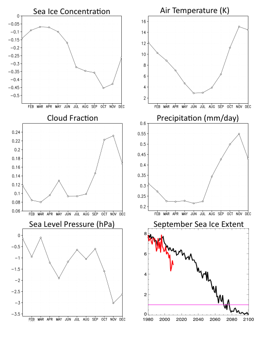
Figure 1: The response of the Arctic annual cycle in the late 21st century to the RCP8.5 greenhouse forcing scenario in CCSM4. Changes in the annual cycle are averaged poleward of 70N over five ensemble members and compared with late 20th century values. (lower right) Evolution of September NH ice extent is shown for the model (black) and observations (red). The timing of a seasonally ice-free Arctic Ocean is indicated by the pink line. [from Vavrus Et al. (2011) Journal of Climate]
Recent work indicates that climate models have a positive bias in the strength of the winter-time low-level temperature inversion over the high-latitude northern hemisphere. It has been argued this bias leads to underestimates of the Arctic's surface temperature response to anthropogenic forcing. Here the bias in inversion strength is revisited. The spatial distribution of low-level stability is found to be bimodal in climate models and observational reanalysis products, with low-level inversions represented by a stable primary mode over the interior Arctic Ocean and adjacent continents, and a secondary unstable mode over the Atlantic Ocean. Averaging over these differing conditions is detrimental to understanding the origins of the inversion strength bias. While nearly all of the 21 models examined overestimate the area-average inversion strength, conditionally sampling the two modes shows about half the models overestimate the inversion strength because of geographical biases and half because of errors in the representation of the Arctic boundary layer. The geographic biases are likely tied to errors in the large-scale circulation, and are connected to the distribution of sea-ice which separates the stable and unstable regimes. This analysis improves understanding of this ubiquitous climate model error, and connects the error to different aspects of the models. This can help to focus model development by focusing attention on processes that lead to the errors in inversion strength.
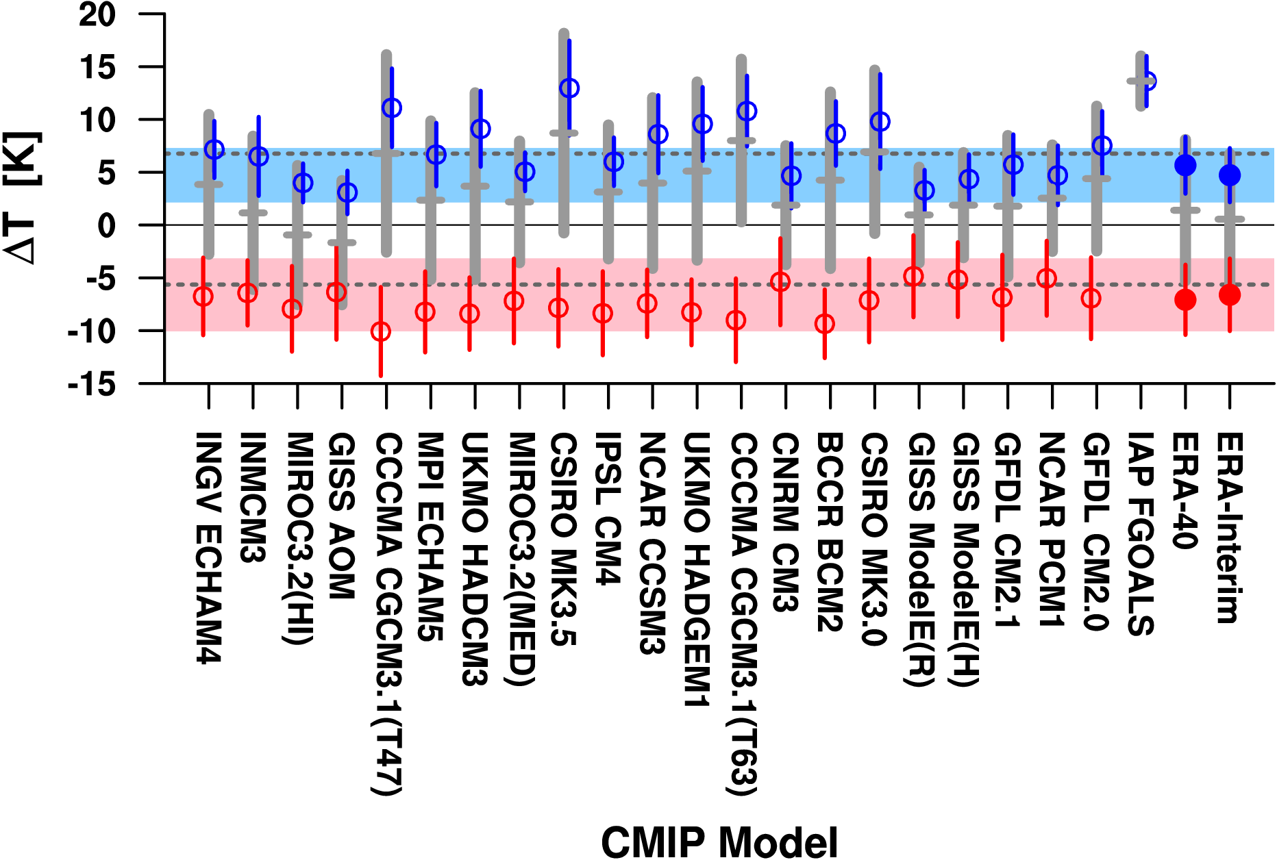
Figure 1: Average inversion strength for the CMIP3 models, ERA-40, and ERA-Interim, (red) unstable, and (blue) stable portion of the inversion strength distribution. Markers show the mean value and whiskers show ±1 standard deviation. The shading shows the ±1 standard deviations of the ERA-Interim values, and lines show the values for the whole Arctic region. Models are organized from left to right by increasing Arctic average sea-ice concentration.
de Boer, G., W. Chapman, J. E. Kay, B. Medeiros, M.D. Shupe, S. Vavrus and J.E. Walsh, 2011: A Characterization of the Present-Day Arctic Atmosphere in CCSM4, J. Climate (in press).
Simulation of key features of the Arctic atmosphere in the fourth version of the Community Climate System Model (CCSM4) is evaluated against observational and reanalysis datasets for the present-day (1981-2005). Surface air temperature, sea level pressure, cloud cover and phase, precipitation and evaporation, the atmospheric energy budget and lower tropospheric stability are evaluated. Simulated surface air temperatures are found to be slightly too cold 15 when compared with ERA-40. Spatial patterns and temporal variability are well simulated. Evaluation of the sea level pressure demonstrates some large biases, most noticeably an under-simulation of the Beaufort High during spring and autumn. Monthly Arctic-wide biases of up to 13 mb are reported. Cloud cover is under-predicted for all but summer 19 months, and cloud phase is demonstrated to be different from observations. Despite low cloud cover, simulated all-sky liquid water paths are too high, while ice water path was generally too low. Precipitation is found to be excessive over much of the Arctic compared to ERA-40 and GPCP estimates. With some exceptions, evaporation is well captured by CCSM4, resulting in P-E estimates that are too high. CCSM4 energy budget terms show promising agreement with estimates from several sources. The most noticeable exception to this are TOA fluxes that are found to be too low while surface fluxes are found to be too high during summer months. Finally, the lower troposphere is found to be too stable when compared to ERA-40 during all times of year, but particularly during spring and summer months.
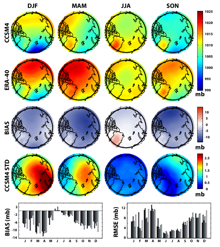
Figure 1: Seasonal mean sea-level pressure (from top to bottom) as simulated by the first CCSM4 ensemble member, from ERA-40, model bias (CCSM4-ERA-40), the standard deviation between all six CCSM4 ensemble members, and CCSM4 bias and RMSE for all six ensemble members (different bars) per month. 70N is indicated by the bold black ring near the perimeter of each map.
Miller, G. H., A. Geirsdottir, Y. Zhong, D. J. Larsen, B. L. Otto-Bliesner, M. M. Holland, D. A. Bailey, K. A. Refsnider, S. J. Lehman, J. K. Southon, C. Anderson, H. Bjornsson, T. Thordarson, 2011: Abrupt onset of the Little Ice Age triggered by volcanism and sustained by sea-ice/ocean feedbacks. Geophys. Res. Let., in review.
The CCSM3 is used to show that abrupt regional cooling in the Arctic during the Little Ice Age (LIA; 1250-1800 AD) could be initiated by explosive volcanism and maintained by subsequent sea-ice/ocean feedbacks. With a favorable initial state, two transient simulations (1150-1625/1700 AD) forced solely by stratospheric volcanic aerosols resulted in a continuously sustained sea-ice expansion following the late 13th Century eruptions, a weakening of the Atlantic Meridional Overturning Circulation (AMOC) by 1350 AD, and an anomalously cold and fresh subpolar gyre that persists through the simulations. The apparent sensitivity of the sea-ice/ocean feedback on the initial state suggests that the state of natural modes of climate variability may determine whether the climate impacts from explosive volcanism extend well beyond their initial primary radiative effects.
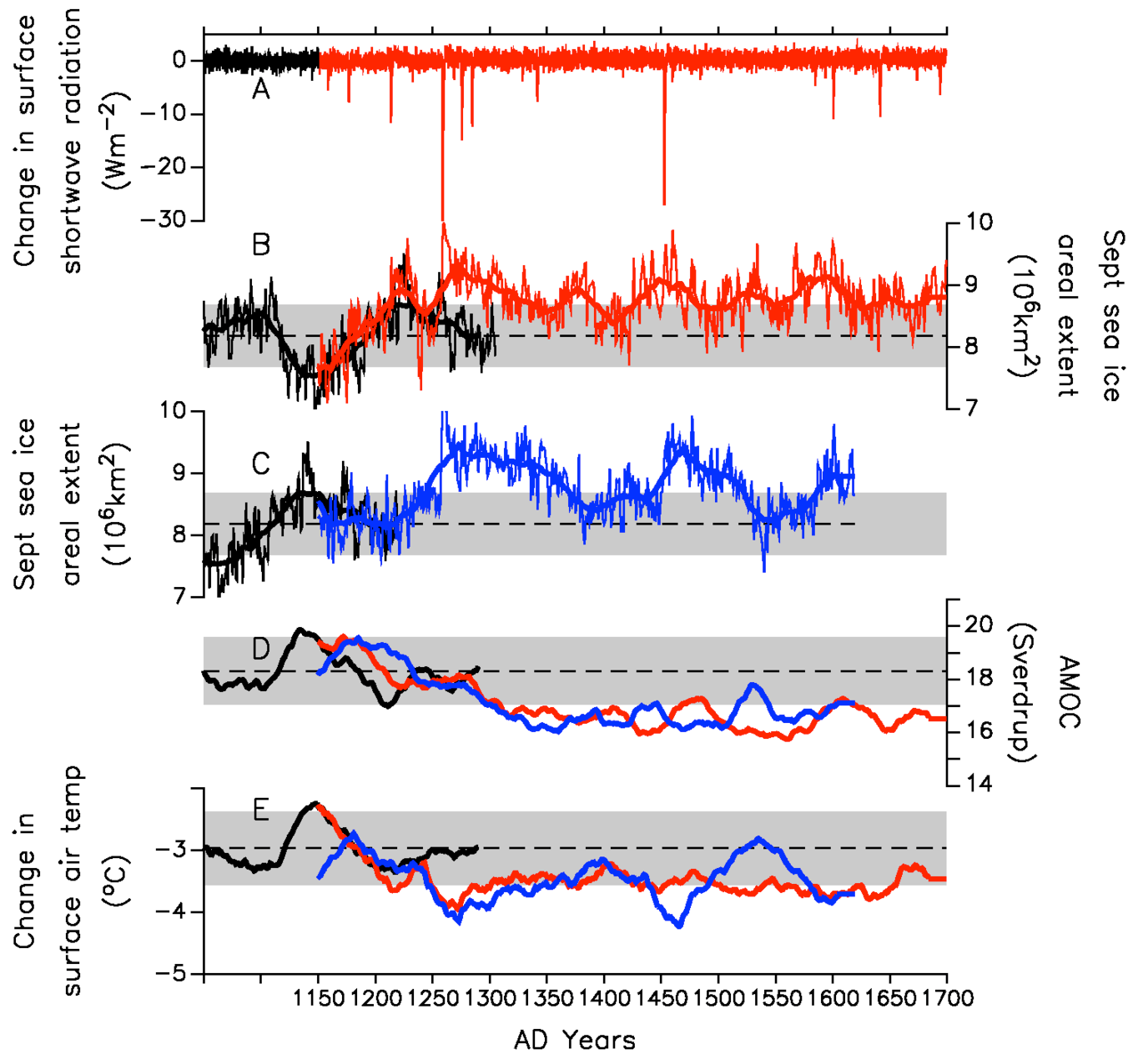
Figure 1: Modeled NH sea ice areal extent, AMOC, change in surface shortwave radiation, and change in surface air temperatures over land area around Atlantic sector of the Arctic. Figure adapted from Miller et al. (2011, in review), Figure 3.
Do changes in atmospheric poleward energy transports explain the large range in Arctic amplification seen in CMIP3 simulations? Definitely not. In fact, models with more polar amplification in 21st century projections show significantly less atmospheric energy transport into the Arctic (Figure 1a). Enhanced Arctic warming weakens the equator-to-pole temperature gradient and decreases atmospheric dry static energy transport, a decrease that often outweighs increases from atmospheric moisture transport. Increasing oceanic transport in most models is positively correlated with Arctic amplification (Figure 1b); however, the increase is too small to compensate the decrease of atmospheric energy transport and the causality of the positive correlation needs further investigation. Model spread in total energy transport cannot explain the model spread in polar amplification; models with great polar amplification must instead have stronger local feedbacks. Because local feedbacks affect temperature gradients, coupling between energy transports and Arctic feedbacks cannot be neglected when studying Arctic amplification.
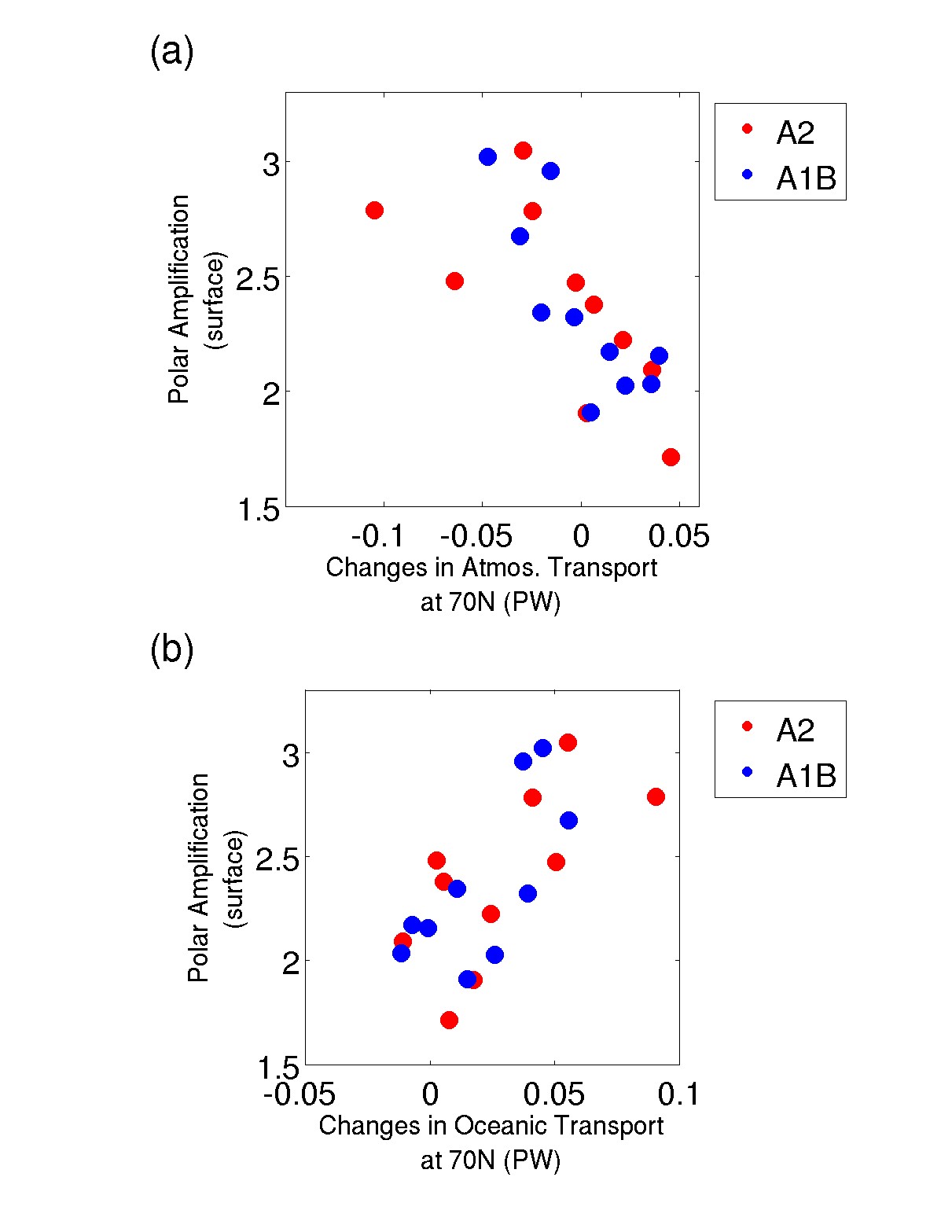
Figure 1: Polar amplification in GCMs versus (a) changes in atmospheric energy transport at 70N (b) changes in oceanic energy transport at 70N. Blue dots are from the A1B scenario, and red dots are from the A2 scenario. Adapted from Hwang et al. 2011, Figure 2.
Jahn, A., K. Sterling, M.M. Holland, J.E. Kay, J.A. Maslanik, C.M. Bitz, D.A. Bailey, J. Stroeve, E.C. Hunke, W.H. Lipscomb, D.A. Pollak, 2011: Late 20th century simulation of Arctic sea ice and ocean properties in the CCSM4. J. Climate, (in press).
To establish how well the new Community Climate System model version 4 (CCSM4) simulates the properties of the Arctic sea ice and ocean, we compared results from a six-member CCSM4 20th century ensemble with available data. We find that the CCSM4 simulations capture most of the important climatological features of the Arctic sea ice and ocean state well, among them the sea-ice thickness distribution, the fraction of multiyear sea ice, and the sea-ice edge. The strongest bias exists in the simulated spring to fall sea-ice motion field, the location of the Beaufort Gyre, and the temperature of the deep Arctic Ocean (below 250 m), which are caused by deficiencies in the simulation of the Arctic sea-level pressure field and the lack of deep-water formation on the Arctic shelves. The observed decrease in the sea-ice extent and of the multiyear ice cover is also well captured by the CCSM4. Looking at the spread between the six ensemble members, we found that the temporal evolution of the simulated Arctic sea-ice cover over the satellite era is strongly influenced by internal variability. One example is the sea-ice thickness at the end of the 20th centurt simulation, which shows differences of over 1 m in the sea-ice thickness in the central Arctic. Another example is the trends in the September sea-ice extent, with one ensemble member showing an even larger negative trend in the September sea-ice extent over 1981–2005 than observed, while two ensemble members show a very small and not statistically significant trend over the same period. This highlights that it is important to compare the observational records not just with the ensemble mean, but also with individual ensemble members, due to the strong imprint of natural variability.
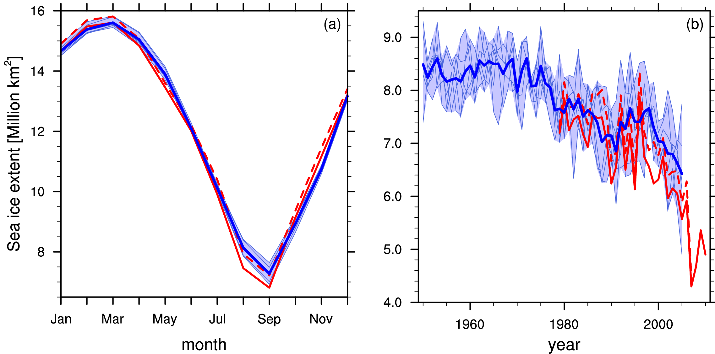
Figure1: a) Climatological seasonal cycle (1981-2005) and (b) timeseries of the sea-ice extent from satellite data (red lines) and from the CCSM4 (blue lines). The CCSM4 ensemble mean is shown in blue, and the spread between the ensemble members is shown by the shaded area, with individual ensemble members shown as thin blue lines. To show the spread in the satellite data due to the use of different retrieval algorithms, we plotted the NSIDC sea-ice extent from Fetterer et al. (2002) as solid red line and the bootstrap sea-ice extent calculated from the sea-ice concentrations from Comiso 1999 as dashed red line. The sea-ice extent is calculated as the area with a sea-ice concentration of 15% or more, and in the satellite data gap around the North Pole the area is assumed to be covered by at least 15% at all times.
Landrum, L., M. M. Holland, D. P. Schneider, and E. Hunke, 2011: Antarctic sea ice climatology, variability and late 20th- Century change in CCSM4. J. Climate (in revision).
The mean modeled Antarctic Sea Ice concentration (SIC) is too extensive in all months compared to late 20th Century observations, the mean modeled ice cover in CCSM4 is too extensive (Figure a). This is in part related to excessively strong westerly winds over ~50°S-60°S, which drive a large equatorward meridional ice transport and enhanced ice growth near the continent. In spite of these biases in the climatology, the model’s sea ice variability compares well to observations (Figure b). The leading mode of austral winter sea ice concentration exhibits a dipole structure with anomalies of opposite sign in the Atlantic and Pacific sectors. These anomalies are related to the timing of ice advance and retreat, are transported eastward with the mean ocean currents, and reoccur over subsequent years due to an imprint of the seasonal ice anomalies on surface ocean conditions. Both the El Niño-Southern Oscillation and the Southern Annular Mode (SAM) project onto the leading mode of sea ice variability and contribute to a significant spectral peak at about four years.
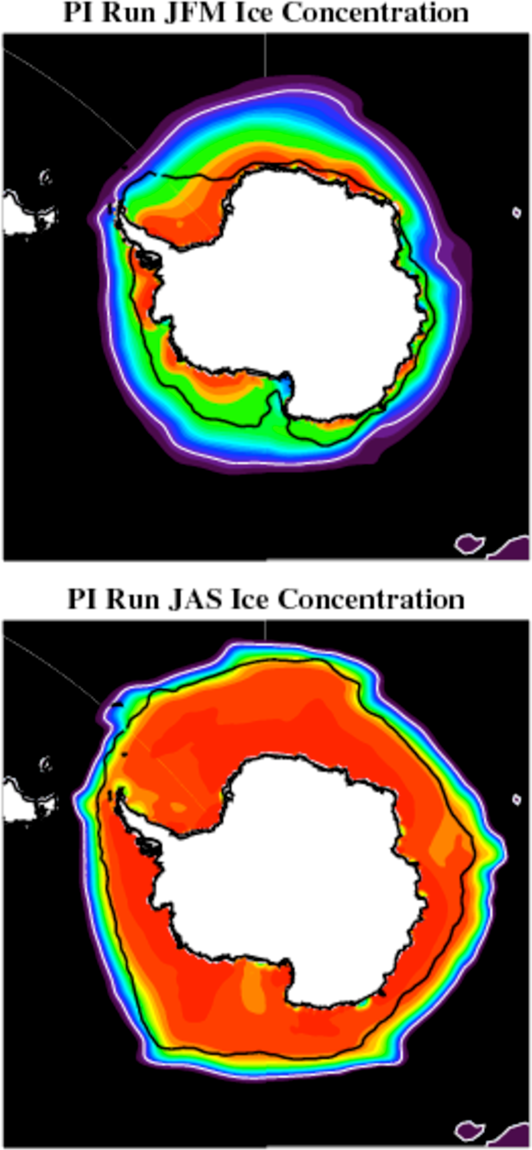
Figure 1: Mean SIC in a) austral summer (JFM) and b) austral winter (JAS). The heavy black contour corresponds to 10% SIC from 1979-2005 satellite data (Comiso, 1990, updated).
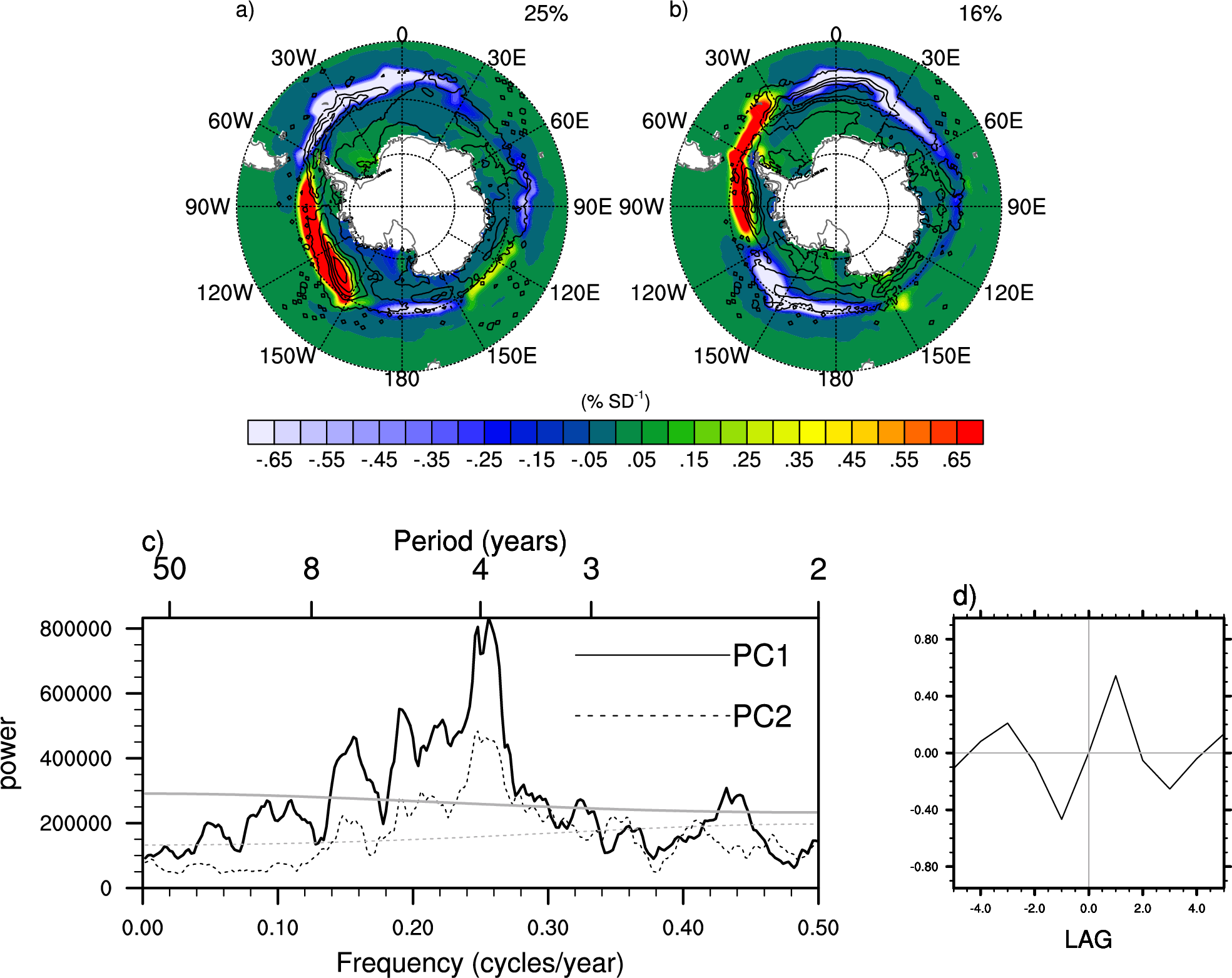
Figure 2: Wintertime (JAS) SIC (a) EOF1 (b) EOF2, c) PC power spectra (gray lines indicate 95% confidence level) and d) correlation of PC1 and PC2. PC1 leads PC2 in the correlation. The black contours in panels (a) and (b) show the corresponding EOFs from observed SIC (Comiso, 1990, updated).