6.9 Numerics

The heat content change within the sea ice over the time interval $t$ to $t'$ corresponding to temperatures $T$ and $T'$, respectively, allowing for temperature dependent heat capacity, thermal conduction (see section 6.6) and internal absorption of penetrating solar radiation, is given by:

$$\int^{T'}_T \rho_i c dT = \rho_i c_o(T'-T) \left(1 + {L_i\mu S \o... ...\partial \over \partial z} k { \partial T \over \partial z} + Q_{SW} \right) dt$$ (6.52)

The heat equation is discretized using a backwards-Euler, space-centered scheme. Using a staggered grid with $T_l$ representing the layer temperature and $k_l$ representing conductivity at the layer interfaces, for interior layers we have

$$\rho_i c_o(T_l^{m+1} - T_l^m) \left(1 + {L_i\mu S_l \over c_o T_l... ...a h^m } - k_l^m { T_l^{m+1} - T_{l-1}^{m+1} \over \Delta h^m } + I^m_l \right),$$ (6.53)

where $\Delta h^m =h^m/L$, the conductivity is

$$k_l^m = k\left({ S_l+S_{l+1} \over 2 } , { T_l^m+T_{l+1}^m \over 2 } \right),$$ (6.54)

and the absorbed solar radiation is

$$I_l^m = I_{0vs} (e^{-\kappa_{vs} l \Delta h^m} - e^{-\kappa_{vs} ... ... + I_{0ni} (e^{-\kappa_{ni} l \Delta h^m} - e^{-\kappa_{ni} (l+1) \Delta h^m}).$$ (6.55)

Figure 6.1: Vertical grid of the sea ice (a) when snow is present and (b) when the ice is snow free; $\Delta h$ is the thickness of an ice layer and $h_s$ is the thickness of the snow layer. The surface temperature in either case is $T_s$. Modified from Bitz and Lipscomb [20].

See Figure 6.1 for a diagram on the vertical level structure.

For a purely implicit backward scheme, $k$ should be evaluated at the $m+1$ time level. However, when $k$ is evaluated at time level $m$, experiments show that the solution is stable and converges to the same solution one gets when evaluating $k$ at $m+1$.

The discrete heat equation for the surface layers is modified slightly from Eq. 6.53 to maintain second-order accuracy for $\partial T/\partial z$. The equation for the bottom layer ($l=L$) is

$$\null \vcenter{\openup\jot \mathsurround=0pt \ialign{\strut\hf... ... - T_{L-1}^{m+1} \over \Delta h^m } + I^m_L \right), \cr\crcr}}$$ (6.56)

where the $L+1$ interface in contact with the underlying ocean is assumed to be at temperature $T_b=-1.8^\circ$C, and where the conductivity is simply $k_{L+1} = k(S_b,T_b)$. The equations for the top surface depend on the surface conditions, of which there are four possibilities, as outlined in Table 6.2.

Table 6.2: Top Surface Boundary Cases

	snow accumulated	melting
case I	yes	no
case II	no	no
case III	yes	yes
case IV	no	yes

6.9.1 Case I: Snow accumulated with no melting

The discrete heat equation for the uppermost layer (i.e, the snow layer) is

$$\rho_s c_s(T_0^{m+1} - T_0^m) = { \Delta t \over h_s^m } \left[ k... ...^{m+1} \over h_s^m } - \beta k_s { T_1^{m+1} - T_s^{m+1} \over h_s^m } \right].$$ (6.57)

The heat equation solver is formulated for the general case where the heat capacity of snow $c_s$ may be specified, although it is taken to be 0. The parameters $\alpha$ and $\beta$ are defined to give second-order accurate spatial differencing for $\partial T/\partial z$ across the changing layer spacing at the snow/ice boundary;

$$\null \vcenter{\openup\jot \mathsurround=0pt \ialign{\strut\hf... ...+ \Delta h^m/2 } {2 \over h_s^m + \Delta h^m} h_s^m.\cr \crcr}}$$ (6.58)

The conductivity at the snow-ice interface is found by equating conductive fluxes above and below the interface;

$$k_1^m={2 k_s k(S_1,T_1^m) \over h_s^m k(S_1,T_1^m) + \Delta h^m k_s}  {h_s^m+\Delta h^m \over 2}.$$ (6.59)

Because $T_s$ is below melting, a flux boundary condition is used, and an additional equation is required in the coupled set:

$$F_o(T_s^{m+1})+\alpha k_s { T_0^{m+1} - T_s^{m+1} \over h_s^m } +\beta k_s { T_1^{m+1} - T_s^{m+1} \over h_s^m }= 0,$$ (6.60)

where $F_o(T_s^{m+1})$ is the sum of all terms on the right-hand side of Eq. 6.2 except $k \partial T / \partial z$. The net surface flux $F_o(T_s^{m+1})$ is approximated as linear in $T_s^{m+1}$; thus

$$F_o(T_s^{m+1})\sim F_o(T_s^m)+\left.{\partial F_o \over \partial T_s}\right\vert _{T_s^m}(T_s^{m+1}-T_s^m).$$ (6.61)

with

$$\left.{\partial F_o \over \partial T_s}\right\vert _{T_s^m} = \le... ...\vert _{T_s^m} + \left.{\partial F_{LH} \over \partial T_s}\right\vert _{T_s^m}$$ (6.62)

To simplify our set of equations, we define

$$\hat c_l^{m+1}= \rho_i \left( c_o + {L_i \mu S \over T_l^{m+1} T_l^m}\right),$$ (6.63)

where the hat implies that $\hat c_l^{m+1}$ depends on $T_l^m$ as well as on $T_l^{m+1}$, and

$$\chi_l^{m+1}= {\Delta t \over \Delta h^m } {1 \over \hat c_l^{m+1}}.$$ (6.64)

Also, let

$$k_l = {k_l^m \over \Delta h^m}.$$ (6.65)

$$l \ge 2$$

$$[-1.0em]$$

$$[-2.0em] k_0 = {k_s \over h_s^m}$$ (6.66)

$$k_1 = {k_1^m \over (\Delta h^m + h_s^m)/2}$$ (6.67)

and suppress the index $m$ for $I_l^m$, so that for interior layers ($l=1...L-1$),

$$T_l^{m+1}-T_l^m =\chi_l^{m+1}\left[k_{l+1}(T_{l+1}^{m+1}-T_l^{m+1}) -k_l(T_l^{m+1}-T_{l-1}^{m+1})+I_l\right]$$ (6.68)
and at the bottom layer

$$[-1.0em] T_L^{m+1}-T_L^m =\chi_L^{m+1}\biggl[3k_b(T_b-T_L^{m+1}) -{1 \over 3}k_b(T_b-T_{L-1}^{m+1}) \cr -k_L(T_L^{m+1}-T_{L-1}^{m+1})+I_L\biggr] \cr$$ (6.69)

where $k_b = k_{L+1} / \Delta h^m$. The equation describing the snow layer is written

$$\rho_s c_s (T_0^{m+1}-T_0^m)={\Delta t \over h_s^m } \left[ k_1(T... ...m+1}) -\alpha k_0(T_0^{m+1}-T_s^{m+1}) -\beta k_0(T_1^{m+1}-T_s^{m+1}) \right].$$ (6.70)

Finally, the flux boundary condition becomes

$$F_o(T_s^m)+ \left. {\partial F_o \over \partial T_s} \right\vert ... ...m+1}-T_s^m) = -\alpha k_0(T_0^{m+1}-T_s^{m+1}) -\beta k_0(T_1^{m+1}-T_s^{m+1}).$$ (6.71)

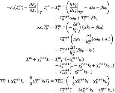
The complete set of coupled equations for case I can be written with all of the terms that explicitly depend on temperature at the $m+1$ time step gathered on the right-hand side:

$$\null \vcenter{\openup\jot \mathsurround=0pt \ialign{\strut\hf... ..._L^{m+1}(1+3 \chi_L^{m+1} k_b + \chi_L^{m+1} k_L ). \cr \crcr}}$$ (6.72)

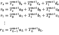
These equations are subsequently related to the following abbreviated form

$$\null \vcenter{\openup\jot \mathsurround=0pt \ialign{\strut\hf... ...\vdots \cr r_L &= T_{L-1}^{m+1} a_L + T_L^{m+1}b_L. \cr \crcr}}$$ (6.73)

The first two rows can be combined to eliminate the coefficient on $T_1^{m+1}$ in the first row, allowing the set to be written in tridiagonal form:

$$\begin{array}{l l l} r = \left[ \begin{array}{c} r_s c_0 - r_... ...m+1} \ T_1^{m+1} \ \vdots \ \end{array} \right]. \end{array}$$ (6.74)

Because the matrix A depends on $\chi_l^{m+1}$, which in turn depends on $T_l^{m+1}$, the system of equations is solved iteratively. An initial guess is used for the temperature dependence of $\chi_l^{m+1}$, and then $\chi_l^{m+1}$ is updated successively after each iteration. Under most conditions the method approaches a solution in less than four iterations with a maximum error tolerance of $\Delta T_{err}$ for $T_l$ with an initial guess of $T_l^{m+1}=T_l^m$.

6.9.2 Case II: Snow free with no melting

Nearly the same method applies when the ice is snow free, except one less equation is needed to describe the evolution of the temperature profile. The equation for the uppermost ice layer is written

$$\null \vcenter{\openup\jot \mathsurround=0pt \ialign{\strut\hf... ...m+1} - T_s^{m+1} \over \Delta h^m } + I^m_1 \right), \cr\crcr}}$$ (6.75)

where $k_1^m=k(S_1,T_1^m)$. After the definitions from Eqs. 6.63-6.65 are applied, Eq. 6.75 becomes

$$T_1^{m+1}-T_1^m=\chi_1^{m+1}\left[k_2(T_2^{m+1}-T_1^{m+1}) -3k_1(T_1^{m+1}-T_s^{m+1}) +{1 \over 3}k_1(T_2^{m+1}-T_s^{m+1})+I_1^m\right].$$ (6.76)

The flux boundary condition follows after linearizing $F_o(T_s^{m+1})$ in $T_s^{m+1}$:

$$F_o(T_s^m)+\left.{\partial F_o \over \partial T_s}\right\vert _{T... ...m+1}-T_s^m) = -3k_1(T_1^{m+1}-T_s^{m+1}) +{1 \over 3} k_1(T_2^{m+1}-T_s^{m+1}).$$ (6.77)

The complete set of coupled equation includes Eqs. 6.72 for layers 2 to L with the following two equations for the surface and upper ice layer:

$$\null \vcenter{\openup\jot \mathsurround=0pt \ialign{\strut\hf... ...}(-\chi_1^{m+1} k_2 - {1 \over 3}\chi_1^{m+1} k_1), \cr \crcr}}$$ (6.78)

which can be written

$$\null \vcenter{\openup\jot \mathsurround=0pt \ialign{\strut\hf... ... r_1 &= T_s^{m+1} a_1 + T_1^{m+1}b_1+ T_2^{m+1}c_1. \cr \crcr}}$$ (6.79)

These two equations can be combined to eliminate the coefficient on $T_2^{m+1}$, allowing the set to be written in tridiagonal form:

$$\begin{array}{l l l} r = \left[ \begin{array}{c} r_s c_1 - r_... ...m+1} \ T_2^{m+1} \ \vdots \ \end{array} \right]. \end{array}$$ (6.80)

As for case I, this system of equations must be solved iteratively.

6.9.3 Case III: Snow accumulated with melting

Case III describes melting conditions in the presence of a snow layer at the surface. Here a temperature boundary condition is used, which simplifies the solution because the first row in Eqs. 6.72 is not needed and $T_s=T_{melt}=0^\circ$C in the second row. Hence the complete set of coupled equations is identical to Eqs. 6.72 for layers 1 to L, with the addition of an equation for the snow layer,

$$\rho_s c_s T_0^m + T_{melt} {\Delta t \over h_s } (\alpha + \beta... ... } (k_1+\alpha k_0 ) \right] - T_1^{m+1} {\Delta t \over h_s } (k_1-\beta k_0).$$ (6.81)

This set of equations can be written in tridiagonal form, without the need to eliminate any terms, as was required in cases I and II. However, the solution must still be iterated.

6.9.4 Case IV: No snow with melting

Like case III, case IV describes melting conditions, but here the sea ice is snow free. Hence, the first two rows of Eqs. 6.72 are not needed, and $T_s=T_{melt}$ for $l=1$. The set of coupled equations comprises those from Eqs. 6.72 for layers 2 to L and the following equation for layer 1:

$$T_1^m + \chi_1^{m+1} I_1^m + T_{melt} \chi_1^{m+1} k_1 {8 \over 3... ...ight) + T_2^{m+1}\left(-\chi_1^{m+1} k_2 - {1 \over 3}\chi_1^{m+1} k_1 \right).$$ (6.82)

As in case III, this set of equations can immediately be written in the tridiagonal form and solved iteratively.

6.9.5 Temperature Adjustment Due to Melt/Growth

Figure 6.2: Diagram showing energy content before (a) and after (b) changing the layer spacing for an ice model with four vertical layers that experiences melt at the top surface and growth at the bottom surface. From [19]

The energy of melting of the ice and snow layers needs to be adjusted when the layer spacing changes after growth/melt, evaporation/sublimation, and flooding (see Figure 6.2). This calculation is only made when CAM 3.0 is coupled to a mixed layer ocean. The adjusted energy of melting is

$$q_l'= \begin{cases}\sum_{k=1}^L w_{k,1} q_k - q_{\rm flood} {z_{i... ...\left. \delta h \right\vert _{\rm basal} \over \Delta h'},0); & l=L \end{cases}$$ (6.83)

where $w_{k,l}$ are weights computed from the relative overlap of layer $l$ with each layer $k$ from the old layer spacing and $\Delta h'$ is the new layer spacing.