The parameterization of non-convective cloud processes in CAM 3.0 is described in Rasch and Kristjánsson [144] and Zhang et al. [200]. The original formulation is introduced in Rasch and Kristjánsson [144]. Revisions to the parameterization to deal more realistically with the treatment of the condensation and evaporation under forcing by large scale processes and changing cloud fraction are described in Zhang et al. [200]. The equations used in the formulation are discussed here. The papers contain a more thorough description of the formulation and a discussion of the impact on the model simulation.
The formulation for cloud condensate combines a representation for condensation and evaporation with a bulk microphysical parameterization closer to that used in cloud resolving models. The parameterization replaces the diagnosed liquid water path of CCM3 with evolution equations for two additional predicted variables: liquid and ice phase condensate. At one point during each time step, these are combined into a total condensate and partitioned according to temperature (as described in section 4.5.3), but elsewhere function as independent quantities. They are affected by both resolved (e.g. advective) and unresolved (e.g. convective, turbulent) processes. Condensate can evaporate back into the environment or be converted to a precipitating form depending upon its in-cloud value and the forcing by other atmospheric processes. The precipitate may be a mixture of rain and snow, and is treated in diagnostic form, i.e. its time derivative has been neglected.
The parameterization calculates the condensation rate more consistently with the change in fractional cloudiness and in-cloud condensate than the previous CCM3 formulation. Changes in water vapor and heat in a grid volume are treated consistently with changes to cloud fraction and in-cloud condensate. Condensate can form prior to the onset of grid-box saturation and can require a significant length of time to convert (via the cloud microphysics) to a precipitable form. Thus a substantially wider range of variation in condensate amount than in the CCM3 is possible.
The new parameterization adds significantly to the flexibility in the model and to the range of scientific problems that can be studied. This type of scheme is needed for quantitative treatment of scavenging of atmospheric trace constituents and cloud aqueous and surface chemistry. The addition of a more realistic condensate parameterization closely links the radiative properties of the clouds and their formation and dissipation. These processes must be treated for many problems of interest today (e.g. anthropogenic aerosol-climate interactions).
The parameterization has two components: 1) a macroscale component that describes the exchange of water substance between the condensate and the vapor phase and the associated temperature change arising from that phase change Zhang et al. [200]; and 2) a bulk microphysical component that controls the conversion from condensate to precipitate [144]. These components are discussed in the following two sections.
As in Sundqvist [169] and Rasch and Kristjánsson [144], the controlling equations for the water vapor mixing ratio, temperature, and total cloud condensate are written as
The controlling equation of relative humidity ![]() , when written on a
pressure surface, can be derived from (4.109) and (4.110) as
, when written on a
pressure surface, can be derived from (4.109) and (4.110) as
| (4.112) | ||
| (4.113) | ||
|
where
| ||
| (4.114) | ||
| (4.115) | ||
| (4.116) | ||
Equations (4.109)-(4.113) are applicable on both the grid
scale and sub-grid scale as long as ![]() ,
, ![]() , and
, and ![]() are
appropriately defined. In the following, a hat denotes variables in
the cloudy portion of a grid box to distinguish them from variables of
the whole grid box, and
are
appropriately defined. In the following, a hat denotes variables in
the cloudy portion of a grid box to distinguish them from variables of
the whole grid box, and ![]() denotes the fractional cloud
coverage. For the portion of the grid box that is cloudy before and
after the calculation of fractional condensation (i.e., the cloudy
area that does not experience clear-cloudy conversion),
equation (4.113) becomes
denotes the fractional cloud
coverage. For the portion of the grid box that is cloudy before and
after the calculation of fractional condensation (i.e., the cloudy
area that does not experience clear-cloudy conversion),
equation (4.113) becomes
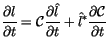
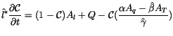
This equation states that the condensation rate is linked with fractional cloudiness change as required by the total water budget. Equation (4.120) is not integrated in the present formulation. Instead, it is used to calculate the condensation rate as follows.
The fractional cloud cover and grid-scale relative humidity are related by
Taking partial derivatives of the equation (4.121) with respect to time gives
| (4.122) | ||
|
and
| ||
| (4.123) | ||
| (4.126) | ||
|
with
| ||
| (4.127) | ||
 |
(4.128) | |
| (4.129) | ||
| (4.130) | ||
|
where
| ||
| (4.131) | ||
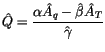
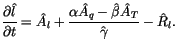
To evaluate ![]() , the cloud routine is called twice each time step
with relative humidity perturbed by one percent (indicated by a
, the cloud routine is called twice each time step
with relative humidity perturbed by one percent (indicated by a ![]() superscript) while holding all other variables in the model fixed.
Thus,
superscript) while holding all other variables in the model fixed.
Thus,
The effects of convection on cloud cover are introduced through the
convective tendencies. Detrainment of cloud water from the
Zhang and McFarlane [199] convection scheme is used as input in the calculation
of ![]() ,
, ![]() and
and ![]() . In the original version of the
Zhang and McFarlane [199] parameterization, the detrained cloud water from
convection was assumed to evaporate.
. In the original version of the
Zhang and McFarlane [199] parameterization, the detrained cloud water from
convection was assumed to evaporate.
The calculation is carried out by categorizing each model grid into one of four cases:
The use of the threshold relative humidity follows from equation (4.121).
The condensation process has been determined by forcing terms and
closure assumptions described in the previous subsection rather than
an approach in which a supersaturation is calculated and CCN can
nucleate and grow. Therefore the whole microphysical calculation
reduces to modeling the process of conversion of cloud condensate to
precipitation. The microscale component of the parameterization
determines the evaporation ![]() and conversion of condensate to
precipitate
and conversion of condensate to
precipitate ![]() .
.
The formulation follows closely the bulk microphysical formulations used in smaller scale cloud resolving models rather than those of Sundqvist [169]. A method based upon cloud resolving models makes an explicit connection between the formation of precipitate and individual physical quantities like droplet or crystal number, shape of size distribution of precipitate, etc. It also separates the various processes contributing to precipitation more strongly, and makes diagnosis more straightforward. Because these quantities must represent an ensemble of cloud types in any given region (or grid volume) the new formulation still involves gross approximations, but it is much easier to control the parameterizations and understand their individual impact when the processes are isolated from each other.
As in Sundqvist [169], the parameterization is expressed in terms
of a single predicted variable representing total suspended
condensate. Within the parameterization, however, there are four types
of condensate expressed as mixing ratios: a liquid and ice phase for
suspended condensate with minimal fall speed (![]() and
and ![]() )
and a liquid and ice phase for falling condensate, i.e. precipitation
(
)
and a liquid and ice phase for falling condensate, i.e. precipitation
(![]() and
and ![]() ). Currently, only the suspended condensates
(
). Currently, only the suspended condensates
(![]() and
and ![]() ) are integrated in time; the other quantities
are diagnosed as described below.
) are integrated in time; the other quantities
are diagnosed as described below.
Before beginning the microphysical calculation, the total condensate is decomposed into liquid and ice phases assuming the fraction of ice is
| (4.132) |
Liquid and ice mass mixing ratios (![]() and
and ![]() ) are independently advected,
diffused, and transported by convection. The detrained liquid from the ZM
convection is all added to the cloud liquid, since the ZM scheme does not have
an ice phase. After the convection and
sedimentation (see below), the liquid and ice are recalculated from the total
cloud condensate
) are independently advected,
diffused, and transported by convection. The detrained liquid from the ZM
convection is all added to the cloud liquid, since the ZM scheme does not have
an ice phase. After the convection and
sedimentation (see below), the liquid and ice are recalculated from the total
cloud condensate
| (4.133) | |||
| (4.134) |
| (4.135) |
The in-cloud liquid water mixing ratio is
| (4.136) |
| (4.137) |
The evaporation of precipitation is computed for each source of precipitation
using the same expressions, following Sundqvist [169]. The
precipitate falling from above can be a mixture of snow and rain. The flux
of total precipitation ![]() on each interface is
on each interface is
| (4.138) |
| (4.139) |
Two bounds are applied to ![]() :
:
Exactly the same procedure is applied to snow,
| (4.140) |
| (4.141) |
The snow production fraction is simple function of temperature
| (4.142) |
Falling precipitation is not permitted to freeze. Snow is produced only by the
assumed snow fraction ![]() in the production term. Snow does not melt unless it
it falls into a layer with
in the production term. Snow does not melt unless it
it falls into a layer with ![]() C, in which case
C, in which case
![]() so that all the snow melts.
so that all the snow melts.
The net heating rate due to freezing, melting and evaporation of precipitation is
| (4.143) |
Cloud liquid and ice particles are allowed to sediment using independent settling velocities, similar to the form described by Lawrence and Crutzen [102]. The liquid and ice settling fluxes are computed at interfaces, from velocities and concentrations at midpoints, using a SPITFIRE solver [145]. The resulting flux at each interface is constrained to be smaller than the mass of liquid or ice in the layer above. This constraint does not allow for particles falling into the layer from above.
Sedimenting particles evaporate if they fall into the cloud free portion of a layer. No bound is applied to prevent supersaturation of the layer. This will be accounted for in the subsequent cloud condensate tendency calculation. Maximum overlap is assumed for stratiform clouds, so particles only evaporate if the cloud fraction is larger in the layer above. The overlapped fraction is
| (4.144) |
The ice velocity ![]() is a function only of the effective radius
is a function only of the effective radius
![]() (see Section 4.8.4 for more information and a plot), which
itself is a function only of
(see Section 4.8.4 for more information and a plot), which
itself is a function only of ![]() . For
. For
![]() m, the
Stokes terminal velocity equation for a falling sphere is used
m, the
Stokes terminal velocity equation for a falling sphere is used
| (4.145) |
For
![]() m, the Stokes formula is no longer valid
and we use a linear dependence of
m, the Stokes formula is no longer valid
and we use a linear dependence of ![]() on
on
![]()
| (4.146) |
The liquid particle velocity depends only on whether the cloud is over land or
ocean, as is true of the liquid effective radius. The net liquid velocity ![]() is
is
| (4.147) |
It is assumed that there are five processes that convert condensate to precipitate:
![]() The conversion of liquid water to rain (PWAUT) follows a
formulation originally suggested by Chen and Cotton [31]:
The conversion of liquid water to rain (PWAUT) follows a
formulation originally suggested by Chen and Cotton [31]:
| (4.148) |
![]() is set to
is set to ![]() over land near the surface,
over land near the surface, ![]() over
ocean, and
over
ocean, and ![]() over sea ice. The number density also varies
with distance from land by a factor equal to the distance to the
nearest land point divided by 1000 km and multiplied by the
cosine of latitude. The provides a sharper transition from land
properties to ocean properties near the poles.
over sea ice. The number density also varies
with distance from land by a factor equal to the distance to the
nearest land point divided by 1000 km and multiplied by the
cosine of latitude. The provides a sharper transition from land
properties to ocean properties near the poles.
The terms ![]() and
and ![]() are the mean volume radii of the
droplets and a critical value below which no auto-conversion is
allowed to take place, respectively.
are the mean volume radii of the
droplets and a critical value below which no auto-conversion is
allowed to take place, respectively. ![]() is the Heaviside function
with the definition
is the Heaviside function
with the definition
![]() for
for
![]() . The volume
radius
. The volume
radius
![]() . The
standard value for the critical mean volume radius at which conversion
begins is
. The
standard value for the critical mean volume radius at which conversion
begins is ![]() m. Baker [9] has shown that this
parameterization results in collection rates that far exceed those
calculated in more realistic stochastic collection models. This is
because the parameterization is based upon a collection efficiency
corresponding to a cloud droplet distribution that has already been
substantially modified by precipitation. Austin et al. [7] suggest that
a much smaller choice is appropriate prior to precipitation
onset. Therefore the parameterization is adjusted by making
m. Baker [9] has shown that this
parameterization results in collection rates that far exceed those
calculated in more realistic stochastic collection models. This is
because the parameterization is based upon a collection efficiency
corresponding to a cloud droplet distribution that has already been
substantially modified by precipitation. Austin et al. [7] suggest that
a much smaller choice is appropriate prior to precipitation
onset. Therefore the parameterization is adjusted by making
![]() when the precipitation flux leaving the grid
box is below 0.5 mm/day.
when the precipitation flux leaving the grid
box is below 0.5 mm/day.
![]() The collection of cloud water by rain from above (PRACW)
follows Tripoli and Cotton [173]
The collection of cloud water by rain from above (PRACW)
follows Tripoli and Cotton [173]
| (4.149) |
![]() The auto-conversion of ice to snow (PSAUT) is similar in
form to that originally proposed by Kessler [85] for liquid
processes and Lin et al. [111] for ice. However, it includes a
temperature dependence similar to that proposed in Sundqvist [169]
The auto-conversion of ice to snow (PSAUT) is similar in
form to that originally proposed by Kessler [85] for liquid
processes and Lin et al. [111] for ice. However, it includes a
temperature dependence similar to that proposed in Sundqvist [169]
| (4.150) |
![]() The collection of ice by snow (PSACI) follows Lin et al. [111],
although it has been rewritten in the form:
The collection of ice by snow (PSACI) follows Lin et al. [111],
although it has been rewritten in the form:
| (4.151) |
The coefficients of the equation (4.152) arise from some
algebraic manipulation of the expressions appearing in
Lin et al. [111]. They in turn depend upon the specification for
parameters describing an exponential size distribution for
graupel-like snow. The parameter values used in Lin et al. [111] are
adopted in the CAM 3.0 implementation. The parameters are a slope
parameter ![]() ; an empirical parameter
; an empirical parameter
![]() controlling the fall speed of graupel-like snow; and the
assumed integrated number density of snow
controlling the fall speed of graupel-like snow; and the
assumed integrated number density of snow
![]() . The
constants appearing in equation (4.152) can be expressed as
. The
constants appearing in equation (4.152) can be expressed as
| (4.153) | ||
| (4.154) | ||
| (4.155) | ||
| (4.156) | ||
| (4.157) | ||
|
and
| ||
| (4.158) | ||
The collection of liquid by snow (PSACW) also follows Lin et al. [111]:
| (4.159) |